Working with vTM Analytics

Overview: vTM Analytics (Enterprise Customers Only)

Services Director supports the configuration and activation of analytics data export on a cluster of Virtual Traffic Managers (vTMs). Each vTM operating at version 17.2 or later supports vTM Analytics. vTM Analytics enables a vTM to send analytics data to an Analytics System.

Collected data can be queried using the vADC Analytics application that is embedded in the graphical user interface of the Services Director VA. This displays tailored graphical reports about the vTMs in its estate.

The use of vTM Analytics is optional, and is only available to customers who purchase an Analytics Resource Pack license.

Currently, the vADC Analytics application is best supported by the Google Chrome browser.

The vTM Analytics process operates as follows:

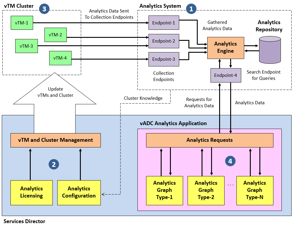
1.Outside of Services Director and the Virtual Traffic Manager, you must install and configure an Analytics System. See Understanding the Analytics System.

Services Director currently supports retrieval of analytics data from the Splunk®1 platform only.

2.On the Services Director, you install an Analytics Resource Pack License, and create all required analytics resources. These are then used to prepare both the cluster and its vTMs for the production of analytics data. See Configuring vTM Analytics on the Services Director.

3.The vTMs in the cluster, now configured to export analytics data, begin to transmit analytics data to the Analytics System, subject to available bandwidth in the Analytics Resource Pack license. See Understanding the Automatic Export of vTM Analytics Data.

4.On the Services Director, the vADC Analytics Application can then query the Analytics System to present the data as a variety of analytics graphs. See Querying vTM Analytics from the Services Director.

Understanding the Analytics System

The vTM Analytics functionality requires an operational Analytics System.

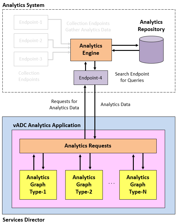
An Analytics System is a grouping of third-party machines, virtual machines, ports, repositories and software that operates collectively to collate analytics data and deliver the required analytics capability.

Currently, the Services Director supports analytics using the Splunk platform.

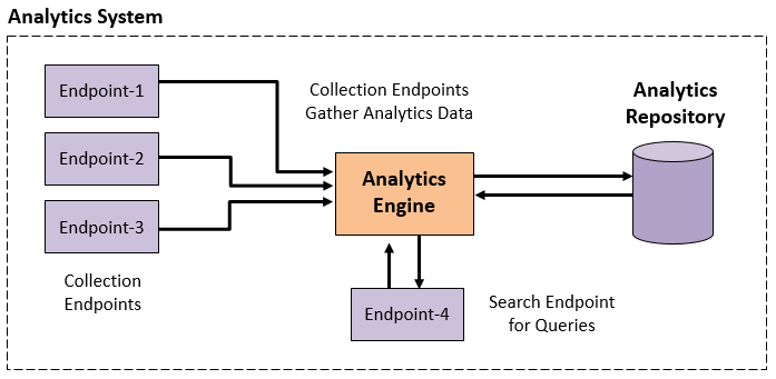
This diagram is generalized; the creation, configuration and operation of the Analytics System will be tailored to your network. These activities are outside the scope of both the Services Director and the Virtual Traffic Manager products.

In general terms, your Analytics System will include:

•An analytics repository to store analytics data.

•An analytics engine that controls the collection, storage and retrieval of analytics data.

•One or more Collection Endpoints. Each collection endpoint receives analytics data from one or more vTMs, including transaction metadata and log data. Typically there will be multiple collection endpoints. Each of these endpoints must be recorded as a Collection Endpoint resource on the Services Director, see Adding a Collection Endpoint Resource to the Services Director.

•One Search Endpoint. This unique endpoint is used by the Services Director to perform queries against analytics data stored in the analytics repository. This endpoint must be recorded as a Search Endpoint resource on the Services Director, see Adding a Search Endpoint Resource to the Services Director.

Once the Analytics System is ready, you can use the Services Director to license and configure vTM analytics data export, see Configuring vTM Analytics on the Services Director.

Configuring vTM Analytics on the Services Director

Before you can configure analytics data export on the vTMs in the estate of the Services Director, you must add an Analytics Resource Pack License to the Services Director, and create all required resources on the Services Director. To do this, you need knowledge of the Analytics System implementation. Specifically, the required endpoints and URLs.

•An Analytics Resource Pack License is required to enable analytics on a fixed number of vTMs. This license defines how many vTMs can be configured to export analytics data to the Analytics System. You must add this to the licenses on the Services Director, see Adding a License to the Services Director.

•Feature Pack resources, each of which references both a Services Director base SKU and an ENT-ANALYTICS add-on SKU. These SKUs are enabled by the Analytics Resource Pack License above. See Adding a Feature Pack to the Services Director.

•Log Export Type resources, each of which identifies the log types that will be exported by the vTM. See Creating a Log Export Type.

•Analytics Profile resources, each of which identifies the types of analytics data (transaction data and logs) exported by the vTM. See Creating an Analytics Profile.

•Collection/Search Endpoint resources, each of which identifies an endpoint in the Analytics System. A single Search Endpoint resource defines where the Services Director will direct queries to in the Analytics System, and a pool of Collection Endpoint resources defines where analytics data will be exported to by the vTMs to the Analytics System. See Adding Analytics Endpoint Resources to the Services Director.

Once the Analytics Resource Pack License and the required resources are in place, you can configure analytics on the Services Director and the vTMs in its estate. To do this, you require:

•A single new Feature Pack for all of the vTMs in the vTM cluster. This must include both a Services Director base SKU and an ENT-ANALYTICS add-on SKU.

•An Analytics Profile to identify the analytics data that will be exported to the Analytics System by the vTMs.

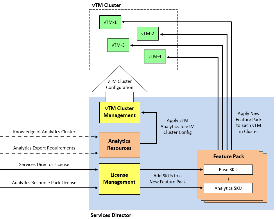
You must then update all vTMs in the cluster to use the new Feature Pack. See Applying a Feature Pack to Registered Instances.

You can then enable analytics on all vTMs in a cluster by applying the required analytics profile to the cluster. You do this from the vTM Clusters page. See Enabling Analytics on a vTM Cluster.

Each vTM is assigned an analytics Collection Endpoint automatically by the Services Director from its pool of Endpoints.

The maximum number of vTMs that can be licensed to produce analytics data is limited only by the available analytics bandwidth in the Analytics Resource Pack License. You can add additional Analytics Resource Pack Licenses to increase this maximum.

Services Director applies the analytics configuration to a single vTM, and vTM cluster replication ensures it reaches all the members of the cluster.

After this process completes, all vTMs in the cluster are configured and licensed for vTM Analytics, and the export of analytics data begins. See Understanding the Automatic Export of vTM Analytics Data.

Understanding the Automatic Export of vTM Analytics Data

Once all vTMs in the cluster are configured and licensed for vTM Analytics (see Configuring vTM Analytics on the Services Director), export of analytics data begins.

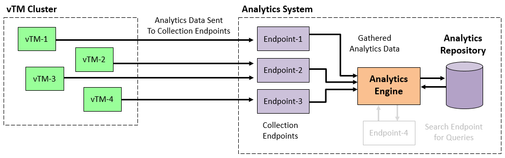
Each vTM transmits the content defined by the cluster’s analytics profile to its assigned collection endpoint on the Analytics System. This data is processed and stored in the analytics repository.

The transmission and processing of analytics data between the vTMs and the Analytics System is outside the scope of Services Director. Refer to the Virtual Traffic Manager documentation.

Once the Analytics Repository starts to accumulate data, the data can be queried by the embedded vADC Analytics application on the Services Director. See Querying vTM Analytics from the Services Director.

Querying vTM Analytics from the Services Director

Analytics data that is stored in an Analytics System can be queried and retrieved by the embedded vADC Analytics application on the Services Director to enable a number of graphical analytics reports. The requests are driven from the user interface for each graph type, and sent to the Search Endpoint for the Analytics System from the Services Director. The retrieved results are displayed within the graphs on the Services Director, and can then be filtered, drilled into, and analyzed. See Configuring vTM Analytics on the Services Director.

Querying of an Analytics System can be performed by all customers who configure a Search Endpoint.

Creating Analytics Resources

After you have added the required Analytics Resource Pack License to the Services Director, you must create the required resources on the Services Director:

•Create a new Feature Pack that includes both a base SKU and a resource SKU that supports vTM analytics. See Adding a Feature Pack to the Services Director.

•Create one or more Log Export Type resources, each of which identifies the log types that will be exported by the vTM. See Creating a Log Export Type.

•Create one or more Analytics Profile resources, each of which identifies the types of analytics data (transaction data and logs) exported by the vTM. See Creating an Analytics Profile.

•Collection/Search Endpoint resources, each of which identifies an endpoint in the Analytics System:

•A single search Endpoint is always used for Services Director queries.

•All other Endpoints are used for data collection. All defined collection Endpoints are handled as a single pool by the Services Director, and allocated to vTMs automatically. See Adding Analytics Endpoint Resources to the Services Director.

Creating a Log Export Type

The Log Export Types page lists all existing log export types in a table. Each entry identifies one or more files that will be sent to the Analytics System by the vTM.

You combine Log Export Types with transaction settings to form an Analytics Profile, see Creating an Analytics Profile.

1.Access your Services Director VA from a browser, using its Service Endpoint IP Address.

2.Log in as the administration user. The Home page appears.

3.Click the Catalogs menu, and then click Analytics > Log Export Types.

The Log Export Types page appears. By default, a number of key Log Export Types are installed with the product. The default Log Export Types may be sufficient for your analytics requirements.

4.Click the Add button above the Log Export Types table.

The Add Log Export Type dialog box appears.

5.Enter a Name for the Log Export Type.

This name will appear in the Log Export Types table.

6.(Optional) Select the Appliance Only check box if this is only supported on Virtual Appliance installations of the vTM, and not on software installations.

7.Enter one or more file names or directories as Files.

•Where you want to specify more than one entry, use a space-separated list.

•The asterisk wild card is supported for multiple selections. For example:

/var/log/auth.log*

•The %ZEUSHOME% system variable enables you to specify file structures relative to the vTM's home directory. For example:

%ZEUSHOME%/admin/log/access*

8.Click Apply. The new Log Export Type is added to the Log Export Types table.

9.Repeat this process to create all required Log Export Types.

You must then combine one or more Log Export Types with transaction settings to form an Analytics Profile. See Creating an Analytics Profile.

Creating an Analytics Profile

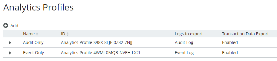
The Analytics Profiles page lists all existing Analytics Profiles in a table. Each entry identifies the Log Export Types and transactions settings that will be sent to the Analytics System by a vTM that uses the Analytics Profile.

You must create all required Log Export Types before you begin, see Creating a Log Export Type.

1.Access your Services Director VA from a browser, using its Service Endpoint IP Address.

2.Log in as the administration user. The Home page appears.

3.Click the Catalogs menu, and then click Analytics > Analytics Profiles.

The Analytics Profiles page appears.

4.Click the Add button above the Analytics Profiles table.

The Add Analytics Profile dialog box appears.

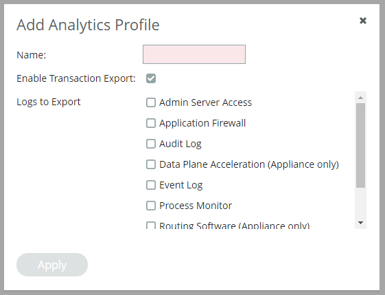
5.Enter a Name for the Analytics Profile.

This name will appear in the Analytics Profiles table.

6.Select the Enable Transaction Export check box to include transaction metadata in the Analytics Profile.

By default, transaction metadata is exported along with any selected logs. If you do not want to export transaction metadata, clear the Enable Transaction Export check box.

7.Select the check box for each required Log Export Type from the Logs to Export list. For example:

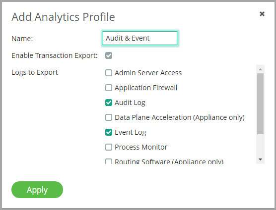
Where a Log Export Type is supported on Virtual Appliance installations of the vTM, this is indicated. For example, the Data Plane Acceleration (Appliance only) Log Export Type. When a Log Export Type is applied to a software vTM, any “Appliance only” Log Export Types are ignored.

8.Click Apply. The new Analytics Profile is added to the Analytics Profiles table.

9.Repeat this process to create all required Analytics Profiles.

Once you have created all required resources, you can apply an Analytics Profile to one or more vTM clusters. See Enabling Analytics on a vTM Cluster.

Adding Analytics Endpoint Resources to the Services Director

Before you can configure analytics on the vTMs in the estate of the Services Director, you must create an Endpoint resource for each of the endpoints on the Analytics System. This includes:

•A pool of Collection Endpoint resources, each of which describes a collection endpoint in the Analytics System that is used to gather analytics data from the vTM cluster. See Adding a Collection Endpoint Resource to the Services Director.

•A Search Endpoint resource. The endpoint identified by this resource is used by the Services Director to perform queries against gathered analytics data in the Analytics System. See Adding a Search Endpoint Resource to the Services Director.

Adding a Collection Endpoint Resource to the Services Director

A collection endpoint is an element of the Analytics System. Each collection endpoint receives analytics data from one or more vTMs. See Understanding the Automatic Export of vTM Analytics Data.

You must add a Collection Endpoint resource to the Services Director for each collection endpoint in the Analytics System. The Services Director maintains a pool of these resources, and references them when you configure analytics on a vTM cluster from the Services Director.

The Analytics Endpoints page lists all existing Collection Endpoint resources in a table.

1.Access your Services Director VA from a browser, using its Service Endpoint IP Address.

2.Log in as the administration user. The Home page appears.

3.Click the Catalogs menu, and then click Analytics > Analytics Endpoints.

The Analytics Endpoints page appears.

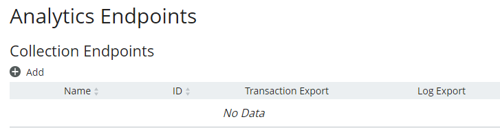
4.Click the Add button above the Collection Endpoints table.

The Add Collection Endpoint dialog box appears.

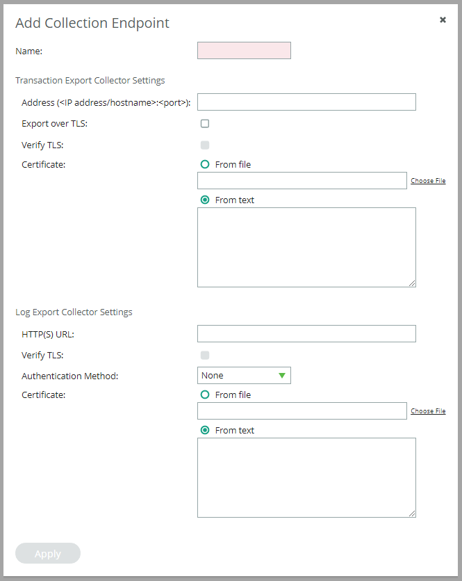
5.Enter a Name for the Collection Endpoint resource.

This name will appear in the Collection Endpoints table.

6.If the collection endpoint will accept transaction metadata, you must now define the Transaction Export Collector Settings for its resource:

•Enter an Address for the collection endpoint in the Analytics System. This takes the form:

You cannot specify a protocol or a filepath.

•If you want Transport Layer Security (TLS) to be used during transaction metadata export, select the Export over TLS check box.

•If the Export over TLS check box is selected, you can choose to verify the TLS connection by selecting the Verify TLS check box.

•If the Export over TLS check box is selected, you must provide an SSL Certificate. To do this, either browse for the required certificate file in the From file property, or paste the contents of the certificate into the From text property.

7.If the Collection Endpoint will accept log data, you must now define the Log Export Collector Settings for its resource:

•Enter an HTTP(S) URL for the collection endpoint in the Analytics System. This takes the form:

The protocol can be either http:// or https://.

If you want Transport Layer Security (TLS) to be used during data export, use the https:// protocol.

•If TLS is used, you can choose to verify the TLS connection by selecting the Verify TLS check box.

•If TLS is used, you must provide an SSL Certificate. To do this, either browse for the required certificate file in the From file property, or paste the contents of the certificate into the From text property.

•Select the required Authentication Method:

•"None". If you select this option, no additional authentication properties are required.

•"Basic HTTP Authentication". If you select this option, you must then specify a Username and Password.

•"Splunk". If you select this option, you must then specify the HEC Token from the Splunk platform.

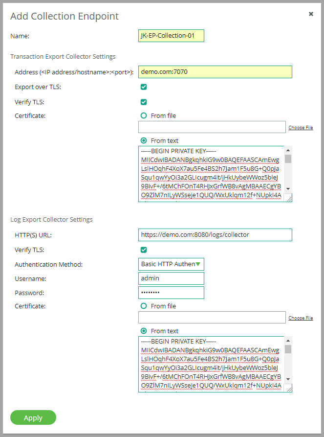
8.Click Apply. The new Collection Endpoint resource is added to the Collection Endpoints table.

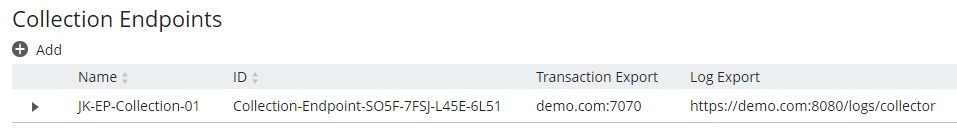
9.(Optional) Expand the Collection Endpoint resource entry to view its full details.

10.Repeat this process to create all required Collection Endpoint resources.

You must also create a single Search Endpoint resource. See Adding a Search Endpoint Resource to the Services Director.

Adding a Search Endpoint Resource to the Services Director

A search endpoint is an element of the Analytics System. The search endpoint receives analytics queries from the Services Director, and returns analytics data to the Services Director. See Understanding the Automatic Export of vTM Analytics Data.

You must add a single Search Endpoint resource to the Services Director to record the properties of the Analytics System's search endpoint.

Querying of an Analytics System can be performed by any customer who configures a Search Endpoint.

Multiple Search Endpoint resources are not supported.

The Analytics Endpoints page displays the Search Endpoints table.

1.Access your Services Director VA from a browser, using its Service Endpoint IP Address.

2.Log in as the administration user. The Home page appears.

3.Click the Catalogs menu, and then click Analytics > Analytics Endpoints. The Analytics Endpoints page appears, which includes a table of Search Endpoints.

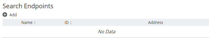
4.Click the Add button above the Search Endpoints table. The Add Search Endpoint dialog box appears.

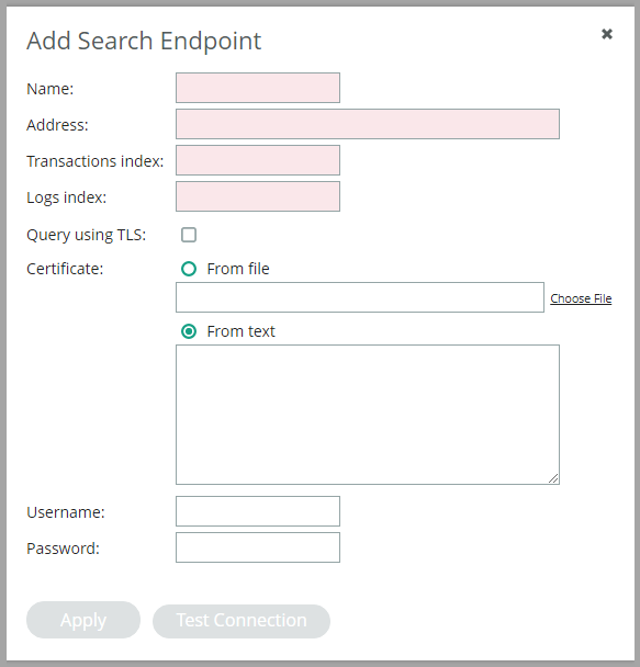
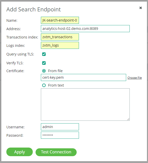
5.Enter a Name for the Search Endpoint resource.

This name will appear in the Search Endpoints table.

6.Enter an Address for the search endpoint in the Analytics System. This takes the form:

You cannot specify a protocol or a filepath.

You can test the connection to this address later in this procedure.

7.Specify the Transactions Index. This is the index used to store transaction data on the Splunk platform. For example, zxtm_transactions.

All transaction data from vTMs should be sent to a specific Splunk index. This index should only be used for transaction data from vTMs.

8.Specify the Logs Index. This is the index used for logs on the Splunk platform. For example, zxtm_logs.

All log data from vTMs should be sent to a specific Splunk index. This index should only be used for log data from vTMs.

9.If you want Transport Layer Security (TLS) to be used during the query, select the Query using TLS check box.

•You can then choose to verify the TLS connection by selecting the Verify TLS check box.

•You must provide an SSL Certificate. To do this, either browse for the required certificate file in the From file property, or paste the contents of the certificate into the From text property.

10.Enter a Username and Password for the query authentication on the Analytics System.

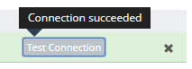
11.(Optional) Click Test Connection to test the search endpoint connection using the specified properties. Success is indicated where the search endpoint can be contacted.

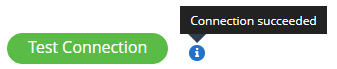
If the test fails, rework your properties and re-test.

12.Click Apply. The new Search Endpoint resource is added to the Search Endpoints table.

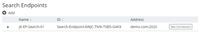
13.(Optional) Expand the Search Endpoint resource entry to view its full details.

14.(Optional) Test a listed search endpoint at any time by clicking the Test Connection button in the Test column of the summary entry for the endpoint. Success is indicated where the search endpoint can be contacted.

You must also create all required Collection Endpoint resources. See Adding a Collection Endpoint Resource to the Services Director.

Enabling Analytics on a vTM Cluster

Once all analytics resources are in place on the Services Director (see Creating Analytics Resources), you can enable vTM analytics on a cluster of vTMs. There are two steps to this process:

•Using the Services Director VA GUI, update each vTM in the cluster to use a Feature Pack that includes a SKU that supports vTM analytics. See Applying a Feature Pack to Registered Instances.

•Using the Services Director VA GUI, update the vTM cluster to use an Analytics Profile. This configures all vTMs in the cluster to generate the analytics data specified by its supported Log Export Types. The vTM is automatically assigned an endpoint in the Analytics System from the pool of Collection Endpoints on the Services Director, and the single Search Endpoint resource. See Adding an Analytics Profile to a vTM Cluster.

Once complete, all vTMs in the vTM cluster will generate analytics data and transmit this data to an assigned collection endpoint in the Analytics System. You are then able to query this data from the Services Director, see Working with Analytics Data on the Services Director.

Adding an Analytics Profile to a vTM Cluster

To enable analytics on all vTMs in a cluster, you must apply an analytics profile to the vTM cluster.

This single action results in the automatic update of every vTM in the cluster by cluster replication, and completes the configuration of analytics from the Services Director.

Before you can enable analytics in a vTM cluster, you must ensure that all vTMs in the cluster use a Feature Pack that supports analytics. See Applying a Feature Pack to Registered Instances.

1.Access your Services Director VA from a browser, using its Service Endpoint IP Address.

2.Log in as the administration user. The Home page appears.

3.Click the Services menu, and then click Services Director > vTM Clusters.

The vTM Clusters page appears.

4.Expand the cluster that you want to update.

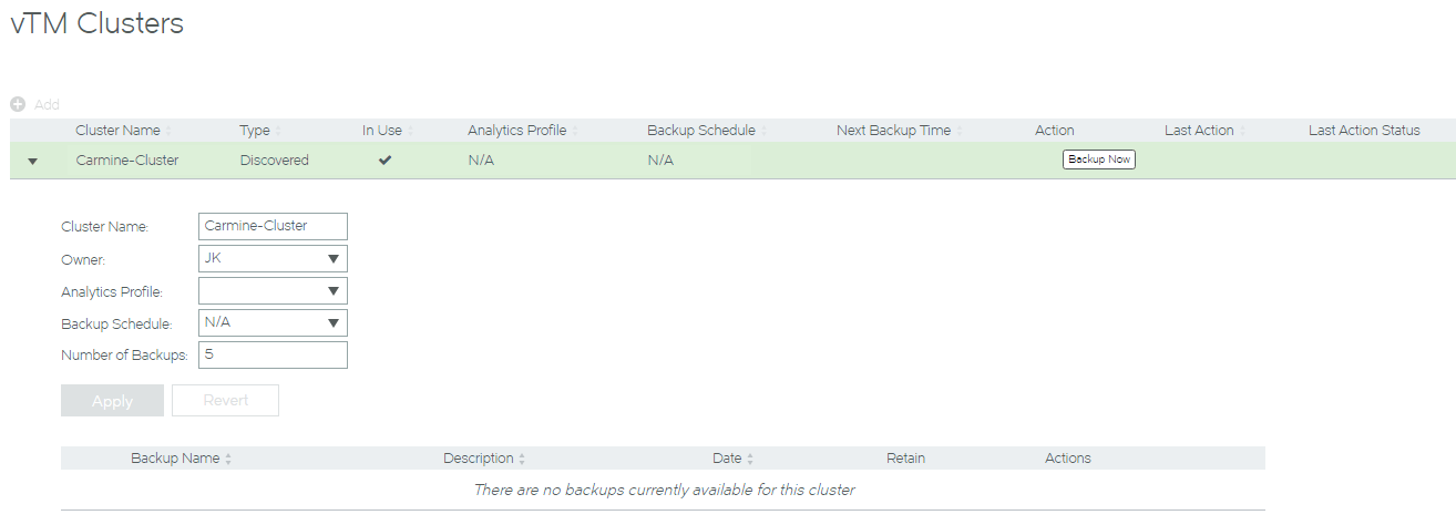
5.Select the required vTM cluster and click Apply.

The cluster update tests all required analytics resources. See Creating Analytics Resources if issues arise.

If all required analytics resources are in place, the cluster updates. After this process is complete, all vTMs in the cluster are updated by cluster replication, and analytics becomes enabled on all vTMs.

Analytics data then starts to accumulate in the Analytics System, and can be queried from the Services Director Analytics interface. See Working with Analytics Data on the Services Director.

Working with Analytics Data on the Services Director

This functionality is available to all Services Director customers.

The Services Director can then use the vADC Analytics Application to query the Analytics System and present the data as a variety of analytics graphs.

•The Analytics Dashboard. This provides a fixed view onto a selection of graphs, to provide high-level information. See Accessing the vADC Analytics Application.

•A number of individual analytics graph types. Each graph type focus on one graphical representation type. This includes:

•Tree graphs. See Using the Sankey Diagram.

•Table graphs. See Using the Table Graph.

•Charts. See Using Charts.

•Dataset graphs. See Using the Dataset View.

Each graph uses a common set of filters to limit data. These filters can be changed at any time:

•The Data Selector. See Choosing a Data Metric.

•The Time Selector. See Choosing a Time Period.

•The Sampling Selector. See Choosing a Sampling Ratio.

•The Component Filter. See Working with the Component Filter.

•The Extended Filter. See Working with the Extended Filter.

Graph-specific behaviours then enable manipulation of displayed data, filtering of results, and drill-down.

•The log data saved from one or more servers. See Working with the Logs View.

Accessing the vADC Analytics Application

The vADC Analytics application provides access to a dashboard and individual analytics graphs.

1.Access your Services Director VA from a browser, using its Service Endpoint IP Address.

2.Log in as the administration user. The Home page appears.

3.Click the Services menu, and then click Analytics: Dashboard and log into the vADC Analytics application using the Services Director credentials.

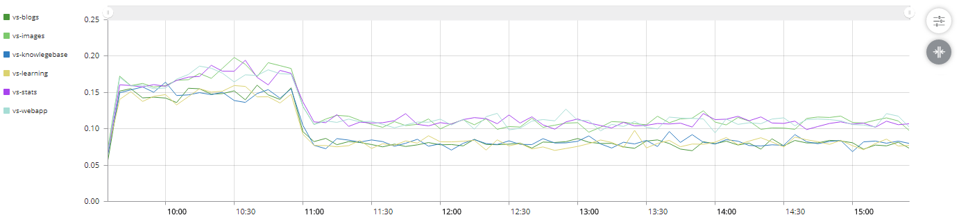
The vADC Analytics application starts in a new window, starting with the Dashboard page. This page presents a view onto a selection of fixed graphs within a single page. Each graph provide a high-level view of your analytics data. For example:

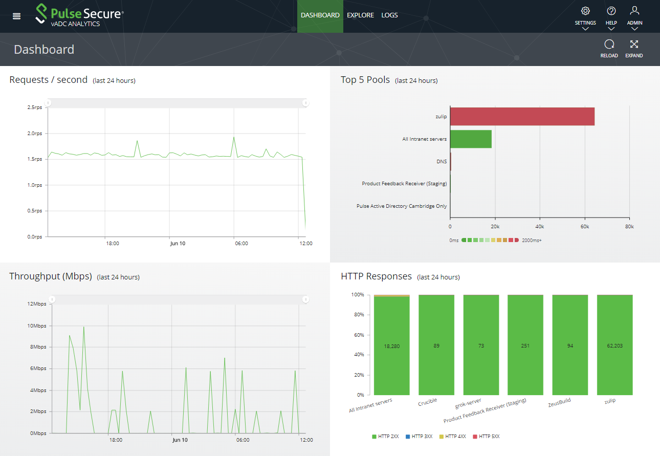
You cannot interact with these graphs. However, you can access individual graph types to perform any required analysis.

The graph types are:

•Tree graphs. See Working with the Extended Filter.

•Table graphs. See Using the Table Graph.

•Charts. See Using Charts.

•Dataset graphs. See Starting the Dataset View.

You can return to the Dashboard at any time by clicking Dashboard.

Returning to the Services Director VA

When you are in the vADC Analytics application, you may want to return to the Services Director VA.

When you start the vADC Analytics application from the Services Director VA, a separate browser tab is started. The tab for the Services Director VA may still be available.

1.In the vADC Analytics application, click the Menu button.

The menu appears.

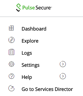
2.Click Go To Services Director.

The Services Director VA appears.

Choosing a Data Metric

The Metric Selector is one of the standard filters that apply to all analytics graph types.

The selected data metric limits the scope of data to a specific measurement type, such as total throughput or requests per second.

The total data for the analytics graph is defined by the combined settings from the Time Selector, the Metric Selector, the Sampling Selector, the Component Filter, and the Extended Filter. Any of these criteria can be changed at any time, and the analytics graph will automatically update to reflect your selections.

Also see Choosing a Time Period, Choosing a Sampling Ratio, Working with the Component Filter and Working with the Extended Filter.

1.Start the vADC Analytics application, see Accessing the vADC Analytics Application.

2.Access the required analytics graph type.

The page for the selected graph type appears. This page includes standard filter controls as well as graph-specific controls.

3.Click the Metric Selector to view all available data metric options.

In this example, you can select total throughput (expressed as Megabits per second), or the number of requests per second.

Some metrics do not support percentiles, and are disabled when percentiles are in use.

4.Click your required data metric.

Once your selection is made, the analytics graph updates automatically, based on the current settings for the Time Selector, Metric Selector, Sampling Selector, Component Filter, and Extended Filter.

Choosing a Time Period

The Time Selector is one of the standard filters that apply to all analytics graph types.

The selected time period limits the scope of data to a specific period of time, which typically ends at the current time. You can also select historical ranges if required.

Also see Choosing a Data Metric, Choosing a Sampling Ratio, Working with the Component Filter and Working with the Extended Filter.

1.Start the vADC Analytics application, see Accessing the vADC Analytics Application.

2.Access the required analytics graph type.

The page for the selected graph type appears. This page includes standard filter controls as well as graph-specific controls.

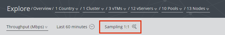
3.Click the Time Selector button to view the list.

A list of fixed time periods appears.

4.(Optional) If you want to include the most recent data in your graph, select the time period that you require from the list. For example, to view data for the last hour, click Last 60 minutes.

5.(Optional) If you want to include a time period that is not specifically listed, or which does not end at the current time, click Select Range. The current list is replaced with a pair of filters that control the start and end of the required time period.

Click on either filter to access standard date/time selection tools.

6.(Optional) To return to a fixed time period, click the Time Selector button and make the required selection.

Once your time period selection is complete, the Component Filter updates automatically to include only those components for which data was received during the requested period. See Working with the Component Filter.

The analytics graph also updates automatically, based on the current settings for the Time Selector, Metric Selector, Sampling Selector, and Extended Filter.

Choosing a Sampling Ratio

The Sampling Selector is one of the standard filters for analytics graph types.

The Sampling Selector does not apply to the Dataset View. See Using the Dataset View.

By default, an analytics graph includes all events for its specified criteria. However, in some situations you might want to retrieve a smaller sampled set of events, instead of retrieving the entire event set:

•You may want to determine the nature of a large data set without processing every event.

For example, for a very large dataset where you wish to study trends, a sampled dataset will be retrieved faster and is likely to indicate all significant trends.

•You may want to perform a quick search to check that expected events are being returned from the current search criteria.

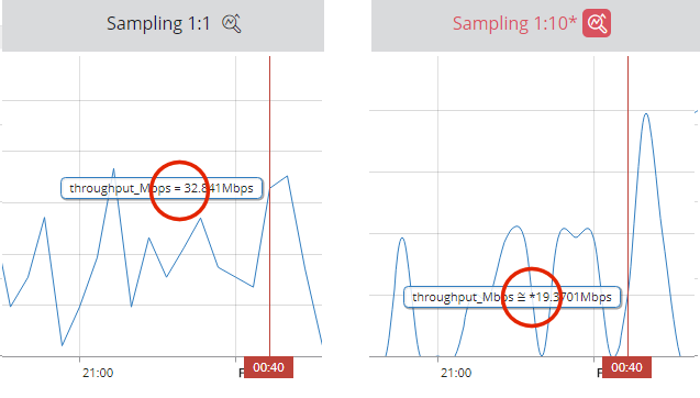
A sampling ratio is the probability of any single event being included in the total result set. For example, if the sample ratio value is 1:100, each event has a 1 in 100 chance of being included in the results. The selection of each event is independent. It is possible that many events will be included from the first 100 events, or that none of these will be included.

If you to re-run a sampling search, different specific results will almost certainly be returned.

A range of sampling ratios from 1:10 to 1:10000 are supported in Services Director. A 1:10 sampling ratio retrieves the most data and is the most representative of source data. A sampling ratio of 1:10000 retrieves the least data and is less representative. A sampling ratio of 1:1 indicates that all data is included. That is, that there is no sampling.

Pulse Secure recommends that you use a 1:1 sampling ratio (that is, there is no sampling) whenever it is practical. If sampling is required, your search should always retrieve as much data as practical. That is, if a 1:10 sampling ratio produces acceptable results, do not proceed to using a 1:100 sampling ratio.

Where analytics events are used to calculate totals (such as Throughput and Requests per Second), sampling should be used with caution. All totals will be approximated for the entire dataset based on the sample, and its heading will be marked with an asterisk to indicate that all numbers are approximate. As the sampling ratio increases, the accuracy of this approximation decreases.

Where a sampled set of results does not include a selected value for a specific Component Filter category, the selected value for the filter is cleared.

Also see Choosing a Data Metric, Choosing a Time Period, Working with the Component Filter and Working with the Extended Filter.

1.Start the vADC Analytics application, see Accessing the vADC Analytics Application.

2.Access the required analytics graph type.

The page for the selected graph type appears. This page includes standard filter controls as well as graph-specific controls.

3.Click the Sampling Selector to view all available data metric options.

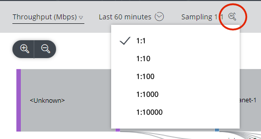
4.Click your required sampling ratio.

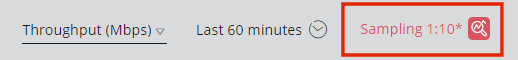
After you have chosen to use sampling, any data that is the result of sampling is indicated, either by:

•The column heading for the value is prefixed by an asterisk.

•The data value itself is prefixed by an asterisk.

•Any "equals" signs are replaced by "approximately equal to" signs.

Once your selection is made, the analytics graph updates automatically, based on the current settings for the Time Selector, Metric Selector, Sampling Selector, Component Filter, and Extended Filter.

Also see Choosing a Data Metric, Choosing a Time Period, Working with the Component Filter and Working with the Extended Filter.

Working with the Component Filter

The Component Filter is one of the standard filters that apply to all analytics graph types.

There is also an extended set of filters, see Working with the Extended Filter.

Also see Choosing a Data Metric, Choosing a Time Period, Choosing a Sampling Ratio, and Working with the Extended Filter.

Understanding the Component Filter

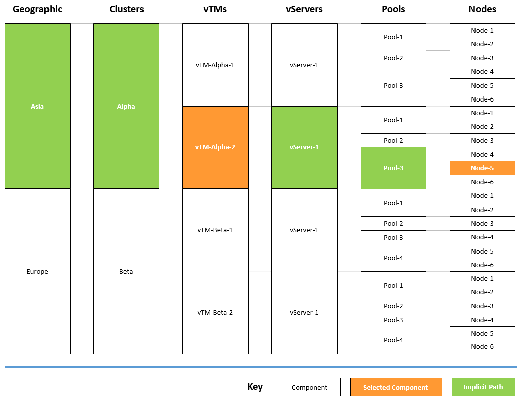
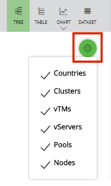
The Component Filter has six component categories (Location, Clusters, vTMs, vServers, Pools and Nodes). You can make selections in all, some or no categories as required.

The Location category can be configured to be based on Continents, Countries or Cities, see Configuring the Location Category.

The Component Filter only lists components for which analytics data is recorded, restricted by:

•The current Time Selector setting. See Choosing a Time Period.

•The current Sampling Selector setting. See Choosing a Sampling Ratio.

•Any selections already made in the Component Filter.

•Any selections made in the Expanded Filter. See Working with the Extended Filter.

When you make a selection, the Component Filter categories can update automatically:

•Where no data is recorded for an individual component after any restrictions (or selections) are applied, the component is omitted from its component category list.

•If you make a selection for a component category, the Component Filter displays and highlights the selection. All other categories (both higher-level and lower-level) for which no selection is made may be updated so that only entries that relate to the most recent selection are listed.

•If no component selection is made for a component category, the current number of components for the category is displayed.

All selections are highlighted:

You can clear a single component type selection by expanding its list and clicking Reset Filter.

You can completely reset the Component Filter at any time by clicking the Reset button:

You can refresh retrieved analytics data by clicking the Reload button. For example, to refresh the analytics data for the Last 6 hours:

You can configure an extended set of filters in addition to the Component Filter by clicking the Filter button, see Working with the Extended Filter.

You can maximize the space within the browser by clicking the Expand toggle.

Understanding Cluster-Level Replication of Components

The configuration of vServers, Pools and Nodes is a cluster-level operation. That is, the configuration of vServers, Pools and Nodes on any vTM is automatically duplicated on all other vTMs in the cluster, using cluster replication. The names and configurations of these resources will be identical.

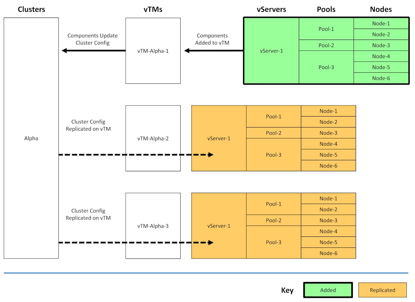
In larger clusters, this will result in large numbers of identically named components within the cluster. To address this issue, all duplicate names are eliminated in the Component Filter. See Understanding Component Filter Categories.

Understanding Component Filter Categories

The Component Filter has six component categories.

•Location category. This category enables you to filter by the geographic location (where known), and can be configured to be based on Continents, Countries or Cities, see Configuring the Location Category.

•Clusters category. Each vTM can be a member of one cluster only, but multiple clusters may be visible from the Services Director. You can make a single cluster selection if required.

•vTMs category. This lists all vTMs within the selected Cluster, or for all listed Clusters if no Cluster is selected. You can make a single vTM selection if required.

•vServers category. This lists all vServers within the selected vTM, or for all listed vTMs if no vTM is selected. You can make a single vServer selection if required.

•Pools category. This lists all Pools within the selected vServer, or for all vServers if no vServer is selected. You can make a single pool selection if required.

•Nodes category. This lists all back-end Nodes within the selected Pool, or for all Pools if no Pool is selected. You can make a single pool selection if required.

Listed components in all categories are restricted automatically by all previous category selections, and by selections to other filters. Only components for which analytics data exists after all selections and filters are applied are included.

All categories can include an entry listed as “None”. This can indicate, for example:

•Incomplete transaction data. That is, a transaction that starts but does not complete, such as might occur during equipment failure.

•Data was retrieved from a cache rather than by forwarding the request.

Cluster-Level configurations such as vServers, pools and nodes will result in repeated component names across all vTMs in a cluster. Component names are not repeated within a category list. A single selected component can refer to many actual components, which can be further explored by making additional selections. See Understanding Cluster-Level Replication of Components.

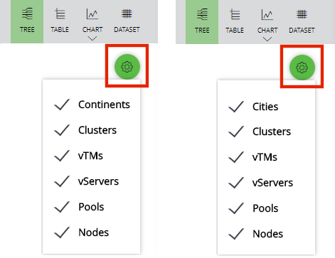
Configuring the Location Category

The Location category enables you to filter by the geographic location of the remote client IP address (where this can be determined). The geographic location can be based on Continents, Countries or Cities.

Where the geographic location of a remote client IP address cannot be identified, such as in a private network, the data is added to a generic Location category grouping called <Unknown>.

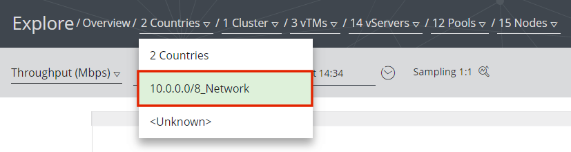
Data from the following standard private networks (as defined by the Internet Assigned Numbers Authority) can be included as a named Location category grouping.

•10.0.0.0/8. This represents the reserved address for 24-bit subnetworks (class A network).

•172.16.0.0/12. This represents the reserved address for 20-bit subnetworks (class B network).

•192.168.0.0/16. This represents the reserved address for 16-bit subnetworks (class C network).

When any of these options are selected, their network can appear in the Location category of the Component Filter. For example:

Configuring the Location Category

1.Click Settings on the toolbar to access the analytics settings.

2.On the pull-down menu, click Geo IP Settings.

The Geo IP Settings dialogue box appears.

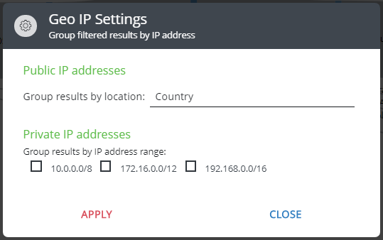
3.Under Public IP addresses, select the required geographical grouping. That is, Continents, Countries or Cities.

4.Under Private IP addresses, select any required standard private networks. That is, 10.0.0.0/8, 172.16.0.0/12 or 192.168.0.0/16.

5.Click Apply.

Example 1: Hierarchic Selection

When you use the Component Filter as a hierarchy, you make left-to-right selections to narrow the scope of a graph to specific components. For example:

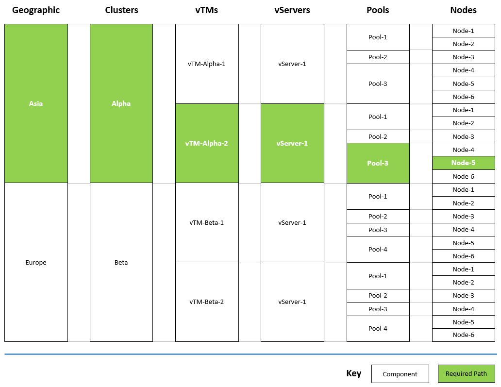
In this example, analytics data exists for all end-to-end paths shown, taking into account the selected time range (see Choosing a Time Period). The required end-to-end path is marked in green; data that was created for this path is required for an analytics graph.

To deliver the required information to the graph, you can use the Component Filter to select the components on the path, one at a time, working left-to-right. The listed options adjust automatically as each selection is made.

For this example:

1.Expand each category in turn and examine the lists. Components for all possible paths are shown:

•There are two continents in the Location category.

•There are two clusters, each of which is in a separate continent.

•There are four vTMs across the two clusters.

•There is one listed vServer. There are four vServers in total across the four vTMs, but there is a single repeating name because of cluster replication. All duplicates are removed. See Understanding Cluster-Level Replication of Components.

•There are four pools. There are fourteen pools in total across the four vTMs, but there are repeating names because of cluster replication. All duplicates are removed.

•There are six nodes. There are 24 nodes in total across the four vTMs, but there are repeating names because of cluster replication. All duplicates are removed.

2.Expand the Location category. Two continents are listed: Asia and Europe. Select Asia,

3.Expand the Clusters category. Two clusters are listed: Alpha and Beta. Select Alpha.

4.Expand the vTMs category. Only the two vTMs in the Alpha Cluster are listed: vTM-Alpha-1 and
vTM-Alpha-2. Select vTM-Alpha-2.

5.Expand the vServers category. Only vServer-1 is listed, as this is the only vServer in the selected vTM. Select vServer-1.

6.Expand the Pools category. Three pools are listed, as these are the pools within the selected vTM:
Pool-1, Pool-2 and Pool-3. Select Pool-3.

7.Expand the Nodes category. Three nodes are listed, as these are the nodes within the selected vTM: Node-4, Node-5 and Node-6. Select Node-5.

All selections are now complete. The analytics graph will use all data for the pathway between the Asia continent and Node-5 on vTM-Alpha-2. This represents an end-to-end connection.

The analytics graph updates after every selection.

You can also reach the same result using a different number of Component Filter selections, using a flexible selection approach. See Example 2: Flexible Component Selection.

Example 2: Flexible Component Selection

When you use the Component Filter to explore analytics data, you can select from any component category at any time, subject to restrictions placed by previous selections.

For example, here is a possible hierarchy of components:

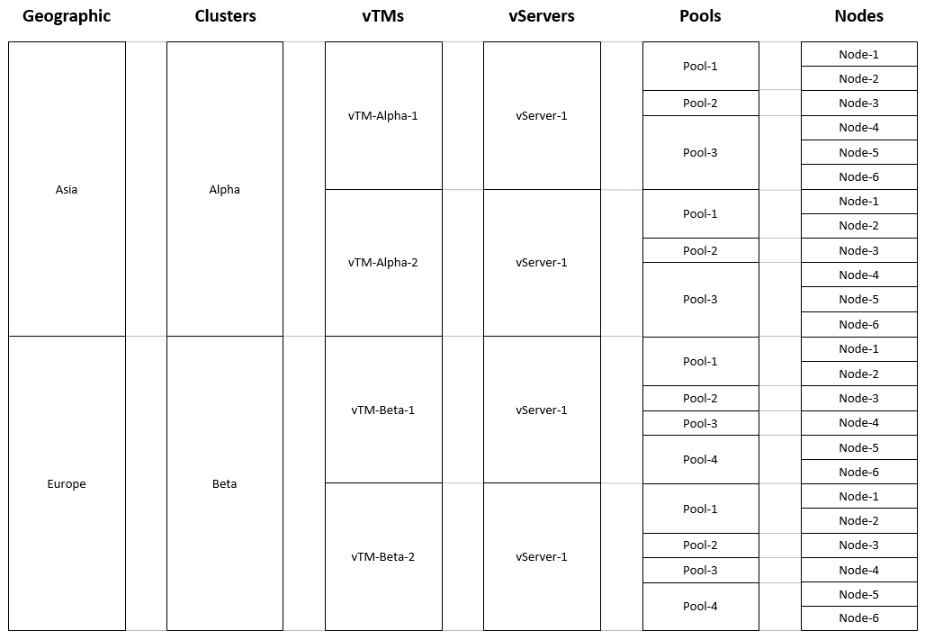
In this example, analytics data exists for all end-to-end paths shown, taking into account the selected time range (see Choosing a Time Period).

You can explore the analytics data, and view the filtered results, by making selections in any category. For this example:

1.Expand each category in turn and examine the lists. Components for all possible paths are shown:

•There are two continents in the Location category.

•There are two clusters, each of which is in a separate continent.

•There are four vTMs across the two clusters.

•There is one vServer. There are four vServers in total across the four vTMs, but there is a single repeating name because of cluster replication. All duplicates are removed. See Understanding Cluster-Level Replication of Components.

•There are four pools. There are fourteen pools in total across the four vTMs, but there are repeating names because of cluster replication. All duplicates are removed.

•There are six nodes. There are 24 nodes in total across the four vTMs, but there are repeating names because of cluster replication. All duplicates are removed.

2.Expand the Nodes category. Six nodes are listed: Node-1, Node-2, Node-3, Node-4, Node-5 and Node-6. Select Node-5. This selection includes all Nodes called Node-5, of which there are four. (see below)

3.Expand the vTMs category. Four vTMs are listed, as each of these vTMs contains a Node called Node-5. Select vTM-Alpha-2.

The two selections have now identified a single pathway between the Asia continent and Node-5 on vTM-Alpha-2. This represents an end-to-end connection.

No more selections are supported without clearing one of the category selections.

The analytics graph updates after each selection.

You can also reach the same result using a different number of Component Filter selections, using an hierarchic selection approach. See Example 1: Hierarchic Selection.

Working with the Extended Filter

The Extended Filter is one of the standard filters that apply to all analytics graph types.

When used, one or more clauses appear in the Extended Filter. All of these must be satisfied for a data item to be included in any analytics graph. For example:

The use of the Extended Filter is described in the following 4 sections:

If you create an Extended Filter clause that is based on one of the standard Component Filter categories, the available values for that category will also be restricted in the Component Filter.

Also see Choosing a Data Metric, Choosing a Time Period, Choosing a Sampling Ratio, and Working with the Component Filter.

Starting the Extended Filter

To start the Extended Filter, click the Filter toggle on the toolbar.

The Extended Filter appears at the bottom of the browser window. When it is started for the first time, it contains no clauses.

To minimize the extended filter, click the Filter toggle again.

Adding Clauses to the Extended Filter

To add one or more clauses to the Extended Filter, perform the following steps.

1.Start the Extended Filter, see Starting the Extended Filter.

The Extended Filter appears at the bottom of the browser window.

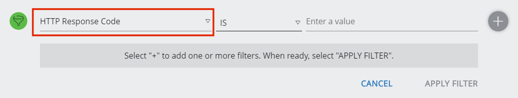
2.In the Extended Filter, either:

•Type the name of the required filter option (field) for the clause, OR

•Expand the list of filter options (fields) and select the required option for the clause.

For example:

See Understanding Extended Filter Clauses for details of clauses.

3.Expand the list of operators, and select the required operator for the clause. For example:

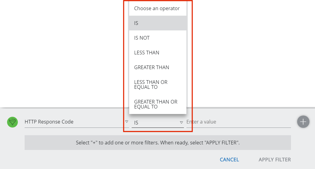
This list is tailored to the selected filter option.

4.Type the required search value for the clause. For example:

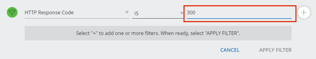
5.Click the + button. The clause is added to the list of clauses. For example:

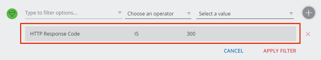
6.Repeat steps 2 to 5 to add more clauses. For example:

Implicit logical operators are applied automatically to the list of clauses, see Understanding Implicit Logical Operators Between Clauses.

The Extended Filter does not display the word “AND”. All listed clauses after the first are related with an AND unless an OR is displayed.

7.Click Apply to apply all listed clauses to the current analytics graph type.

8.(Optional) To minimize the extended filter at any time, click the Filter toggle. When the Extended Filter is populated with one or more clauses, it minimizes to the bottom of the browser window and remains visible. For example:

Understanding Extended Filter Clauses

The Extended Filter is specified as a list of user-defined clauses. Each clause identifies:

•A field in the transaction data that was exported by a vTM to the analytics repository.

•A condition that relates to the field.

•A value for the condition.

That is:

<field> <condition> <value>

For example:

Remote Client Port IS 123

The supported conditions and values for a clause depend upon the specified field:

•Numeric fields can support one of more of the following conditions:

•IS. For example: Remote Client Port IS 8080

•IS NOT. For example: Remote Client Port IS NOT 8100

•LESS THAN. For example: Transaction Duration LESS THAN 30

•LESS THAN OR EQUAL TO. For example: Transaction Duration LESS THAN OR EQUAL TO 17

•GREATER THAN. For example: Transaction Duration GREATER THAN 23

•GREATER THAN OR EQUAL TO. For example:
Transaction Duration GREATER THAN OR EQUAL TO 40

•IS PRESENT. For example: Transaction Duration IS PRESENT

•IS ABSENT. For example: Transaction Duration IS ABSENT

•String fields support the following conditions:

•IS. For example: Protocol IS “HTTP”

•IS NOT. For example: Protocol IS NOT “FTP”

•CONTAINS. For example: Protocol CONTAINS “TP”

•DOES NOT CONTAIN. For example: Protocol DOES NOT CONTAIN "FT"

•IS PRESENT. For example: Protocol IS PRESENT

•IS ABSENT. For example: Protocol IS ABSENT

•Boolean fields support the following conditions:

•IS. For example: HTTP Response Server Keep Alive IS TRUE

•IS PRESENT. For example: HTTP Response Server Keep Alive IS PRESENT

•IS ABSENT. For example: HTTP Response Server Keep Alive IS ABSENT

The user does not define the logical relationships between the various clauses using explicit logical operators,

Rather, the Extended Filter is subject to implicit logical operators that are imposed automatically by the vADC Analytics Application, see Understanding Implicit Logical Operators Between Clauses.

Understanding Implicit Logical Operators Between Clauses

The user can define one or more Extended Filter clauses to manage the information that is included in analytics graphs. See Understanding Extended Filter Clauses.

The user does not define the logical relationships between extended filter clauses using explicit logical operators, Rather, the Extended Filter clauses are subject to implicit logical operators that are imposed automatically by the vADC Analytics Application.

•All clauses that reference a single field using “IS” or “CONTAINS” operator are automatically related via an implicit OR logical operator. For example, the following clauses reference the same field:

Field-X IS 10

Field-X IS 20

Field-X IS 50

This is equivalent to:

Field-X IS 10

OR Field-X IS 20

OR Field-X IS 50

•All other clauses are automatically related via an implicit AND logical operator. For example:

Field-A GREATER THAN 10

Field-A LESS THAN OR EQUAL TO 20

Field-B IS NOT “Halo”

Field-C IS “CBG”

Field-D IS NOT 66
Field-E IS PRESENT

This is equivalent to:

Field-A GREATER THAN 10

AND Field-A LESS THAN OR EQUAL TO 20

AND Field-B IS NOT “Halo”

AND Field-C IS “CBG”

AND Field-D IS NOT 66

AND Field-E IS PRESENT

•A list of clauses can combine both of these clause types:

Field-X IS 10

Field-X IS 20

Field-A GREATER THAN 10

Field-A LESS THAN OR EQUAL TO 20

Field-B IS NOT “Halo”

Field-C IS “CBG”

Field-D IS NOT 66

Field-E IS PRESENT

Field X IS 50

This is equivalent to (with OR terms grouped together):

(Field-X IS 10

OR Field-X IS 20

OR Field-X IS 50)

AND Field-A GREATER THAN 10

AND Field-A LESS THAN OR EQUAL TO 20

AND Field-B IS NOT “Halo”

AND Field-C IS “CBG”

AND Field-D IS NOT 66

AND Field-E IS PRESENT

In all cases, the resulting extended filter is applied to the analytics graph.

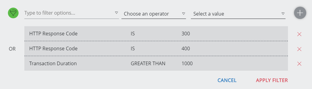
The Extended Filter does not display the word “AND”. All listed clauses after the first are related with an AND unless an OR is displayed. For example:

In this example, the clauses are related as follows:

(HTTP Response Code IS 300 OR HTTP Response Code IS 400)

AND Transaction Duration GREATER THAN 1000
AND HTTP Response Header Content-Type IS PRESENT
AND HTTP Response Header Content-Encoding IS PRESENT

When the Extended Filter is minimized in the browser window, the clauses appear as follows:

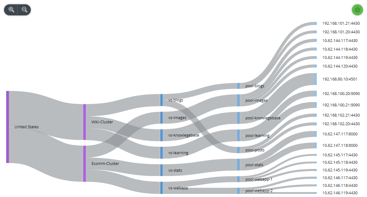
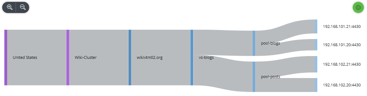
Using the Sankey Diagram

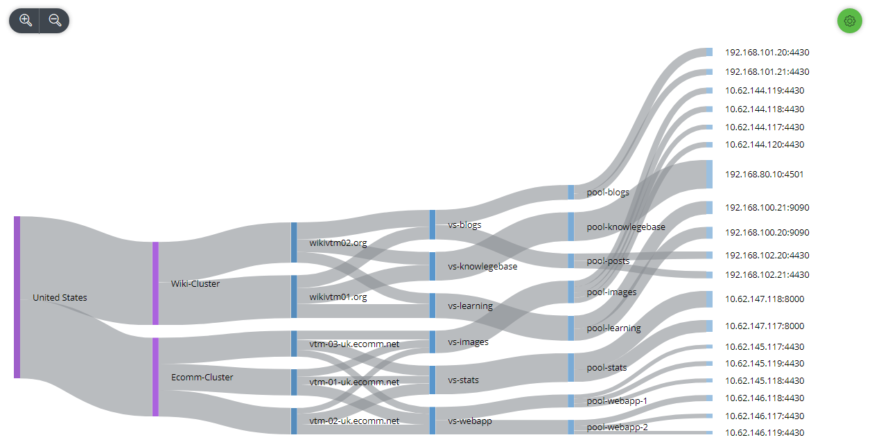
The supported tree graph is a Sankey diagram. This is a specific type of flow diagram, in which the width of the graph lines is proportional to the flow quantity between each pair of points.

For analytics purposes, the width of the line on the Sankey diagram shows proportional flow of the chosen data metric (see Choosing a Data Metric).

Flow is calculated for all end-to-end connections between the geographic areas and nodes in your vTM cluster, and displayed according to included components. For example:

To display a Sankey diagram, see Starting the Sankey Diagram.

Once a Sankey diagram is displayed, you can focus on your analytics data as follows:

•Selecting Included Components for your Sankey Diagram.

•Focusing on a Component in a Sankey Diagram.

•Focusing on a Path in a Sankey Diagram.

You can also update the following controls at any time:

•The Component Filter, see Working with the Component Filter.

•The Metric Selector, see Choosing a Data Metric.

•The Time Selector, see Choosing a Time Period.

The scope of the Sankey diagram updates immediately to include and-to-end connections that meet all selection criteria.

Starting the Sankey Diagram

1.Start the vADC Analytics application, see Accessing the vADC Analytics Application.

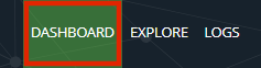
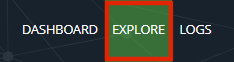
2.Click Explore to access individual analytics graphs.

Alternatively, click the Menu button, and then click Explorer.

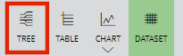
3.Finally, click the Tree graph type.

The required graph type appears.

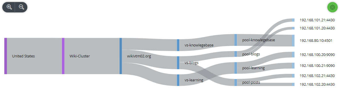
Selecting Included Components for your Sankey Diagram

By default, the Sankey diagram includes all six component categories:

•Location. This can be configured to be based on Continents, Countries or Cities, see Configuring the Location Category.

Where data events are collected for more than ten country/city locations, each location is ranked according to the number of data events collected. The top ten locations are displayed individually in the Sankey diagram, and all locations after the tenth are displayed as a single entry named "Rest of the World".

•Clusters

•vTMs

•vServers

•Pools

•Nodes

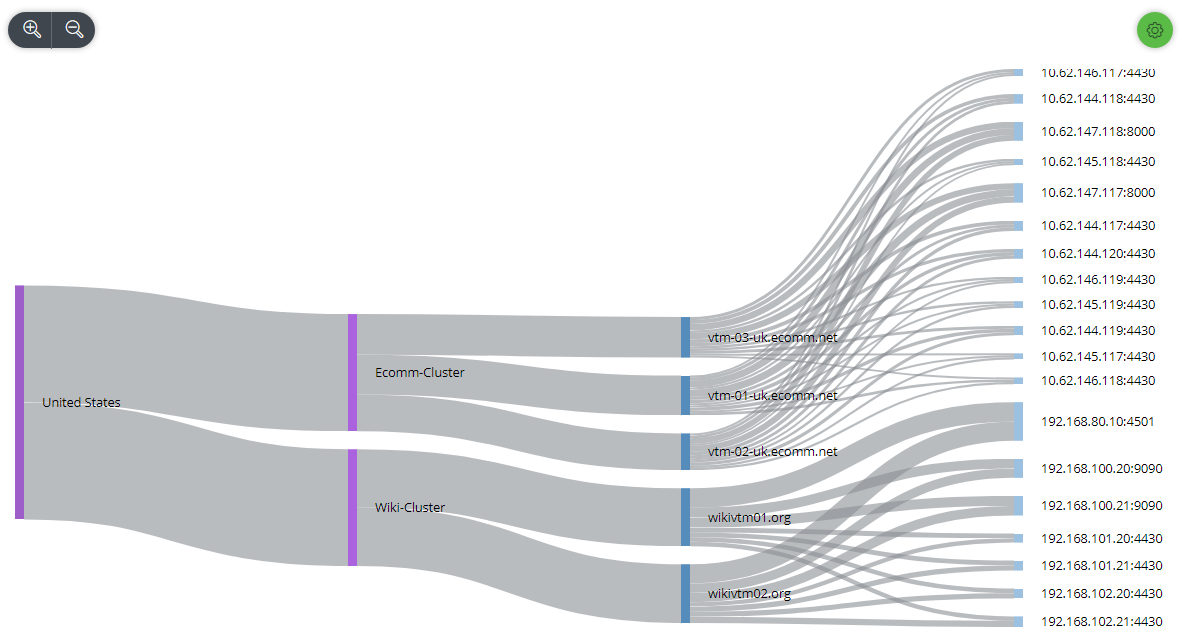
You can exclude specific component types from the diagram if required.

1.Display a Sankey diagram. See Starting the Sankey Diagram. For example:

2.Click the Settings button to display a check list of component types. For example:

In this example, the Location category is set to the Countries setting. This can also be set to Continent or City, see Configuring the Location Category.

3.Select a component type to include/exclude it.

For example, after excluding vTMs:

For example, after excluding both vServers and pools:

Focusing on a Component in a Sankey Diagram

You can focus on a specific component in the Sankey diagram, which updates the graph to include only those end-to-end connections that include the selected component.

1.Display a Sankey diagram. See Starting the Sankey Diagram. For example:

2.In the Sankey diagram, hover the mouse pointer over the required component to display:

•An indication of all end-to-end paths passing through the node.

•The name of the node. For example:

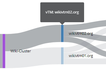
3.Click the node. The Sankey diagram updates to include all end-to-end connections that include the selected component. For example:

You can also focus on a specific path in the Sankey diagram, see Focusing on a Path in a Sankey Diagram.

Focusing on a Path in a Sankey Diagram

You can focus on a single path in the Sankey diagram, which updates the graph to include only those end-to-end connections that include the selected node.

1.Display a Sankey diagram. See Starting the Sankey Diagram. For example:

2.In the Sankey diagram, hover the mouse pointer over the required path to see its details. For example:

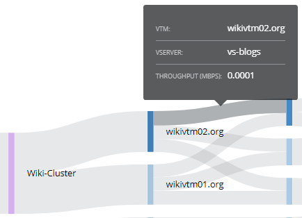
When sampling is applied to the dataset, this is indicated by an asterisk prefix on the heading. For example, Throughput is replaced by *Throughput.

3.Click the path. The Sankey diagram updates to include all end-to-end paths that include the selected path. For example:

You can also focus on a specific component in the Sankey diagram, see Focusing on a Component in a Sankey Diagram.

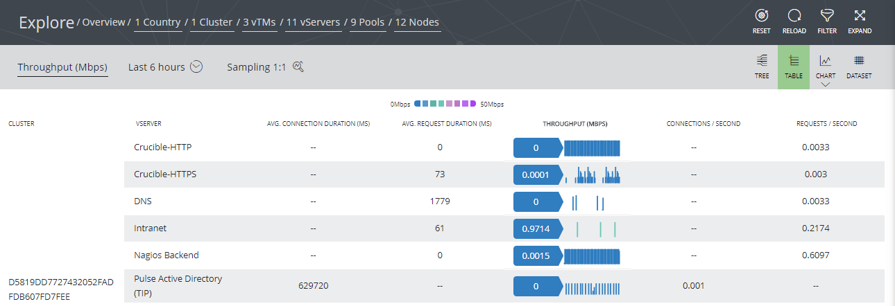
Using the Table Graph

The supported Table Graph is a per-vServer summary of all of the available metrics. The graph also includes a sparkline that shows trends in the currently data for all selected criteria. For example:

To display a Table Graph, see Using Charts.

You can also update the following controls at any time:

•The Component Filter, see Working with the Component Filter.

•The Metric Selector, see Choosing a Data Metric.

•The Time Selector, see Choosing a Time Period.

The scope of the Table Graph updates to include and-to-end connections that meet all selection criteria.

Starting the Table Graph

1.Start the vADC Analytics application, see Accessing the vADC Analytics Application.

2.Click Explore to access individual analytics graphs.

3.Finally, click the Table graph type.

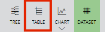
The required graph type appears.

Understanding the Table Graph

The Table Graph can include the following measurements:

•Cluster

•vServer

•Average Connection Duration (milliseconds). This property contains a connection duration measurement for a protocol such as TCP.

•Average Request Duration (milliseconds). This property contains a request duration measurement for a protocol such as HTTP or HTTPS.

•Throughput (MBits per second)

•Connections per Second.

•Requests per Second.

Some of these measurements will be blank, depending on the protocol in use, and on the selected data metric, see Choosing a Data Metric.

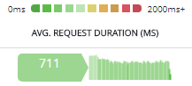
Where sampling is used, this is indicated by an asterisk prefix in the column headings. For example:

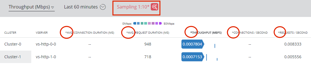
The measurement that matches your selected data metric (see Choosing a Data Metric) is supplemented with a “sparkline” graphic. This graphic visually summarizes measurements across the required time range, with an overall colour coding. For example:

Using Charts

The Primary Chart displays values for the current data metric over time. Optionally, this can be split by component type.

A set of secondary graphs on tabs underneath the Primary Chart provide deeper analysis and comparisons with the main chart. These are:

•The Comparative Analysis tab, see Performing Comparative Analysis.

•The Alternative Views tab, see Viewing the Horseshoe Diagram.

•The HTTP Response Codes tab, see Viewing HTTP Response Codes.

•The Top Events tab, see Viewing Top Events.

Starting the Chart

1.Start the vADC Analytics application, see Accessing the vADC Analytics Application.

2.Click Explore to access individual analytics graphs.

3.Click the Chart graph type.

4.Select the required graph type, see Chart Types.

The required graph type appears.

Chart Types

There are four chart types supported, each of which is accessed from the Chart pull-down menu.

•Line charts. For example:

Line charts support splits. For example, if split by vTM:

•Bar charts. For example:

Bar charts support splits. For example, if split by vTM:

When splits are used, bar charts are presented as stacked data.

•Simple area charts. For example:

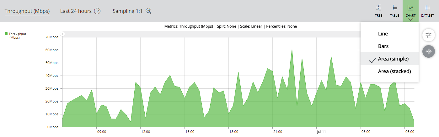
Area charts support splits. For example, if split by vTM:

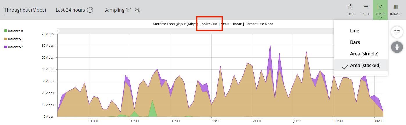
•Stacked area charts. This chart type requires split data, as different data sets are cumulatively stacked vertically.

For example:

Using a Logarithmic Vertical Axis

A logarithmic scale is a nonlinear scale that is used when there is a large range of quantities.

If an axis uses a logarithmic scale, each displayed value is ten times bigger than the one beneath it, as it is based on orders of magnitude; large values become closer together visually, and more differentiation is possible for values that are closer to zero.

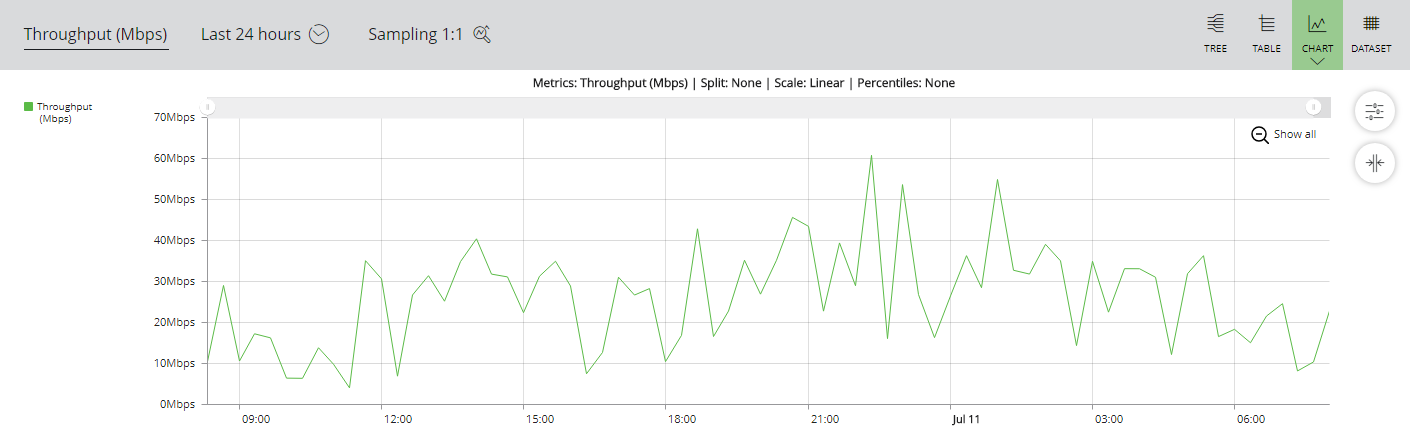
Linear Scales and Logarithmic Scales

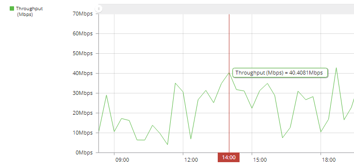
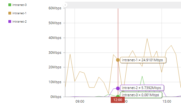
The following diagrams compare the same data displayed using linear and logarithmic scales.

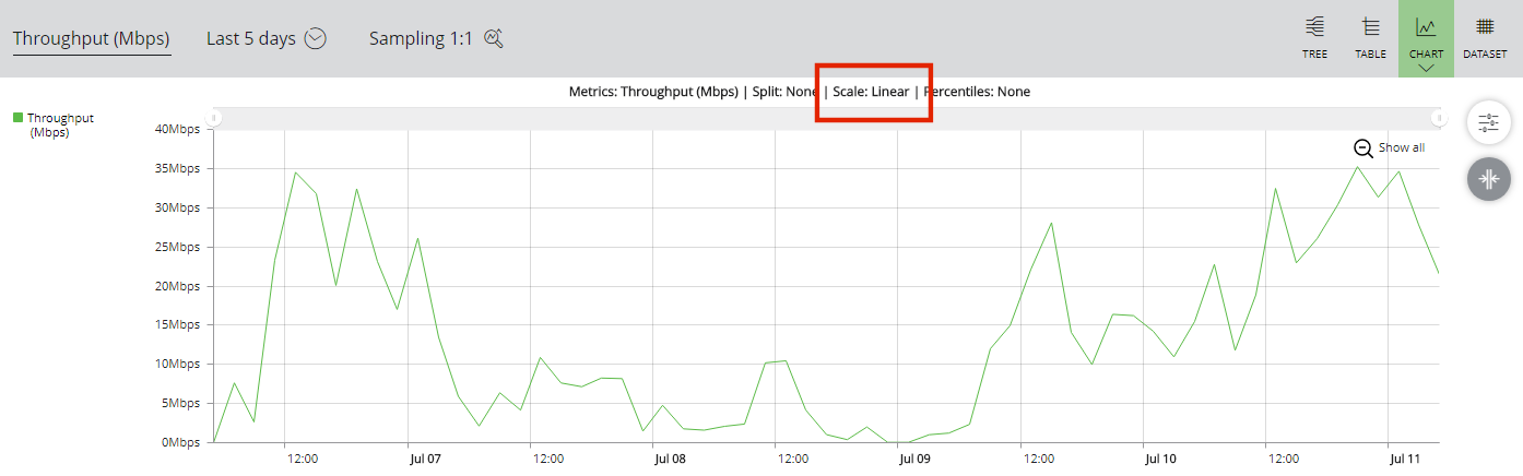
In this example:

•The vertical axis is marked from 0Mbps to 40Mbps in linear 10Mbps increments.

•The smaller values (many less than 1Mbps) are hard to read (and to differentiate from zero/missing), because of the huge difference between them and the larger values on the linear scale.

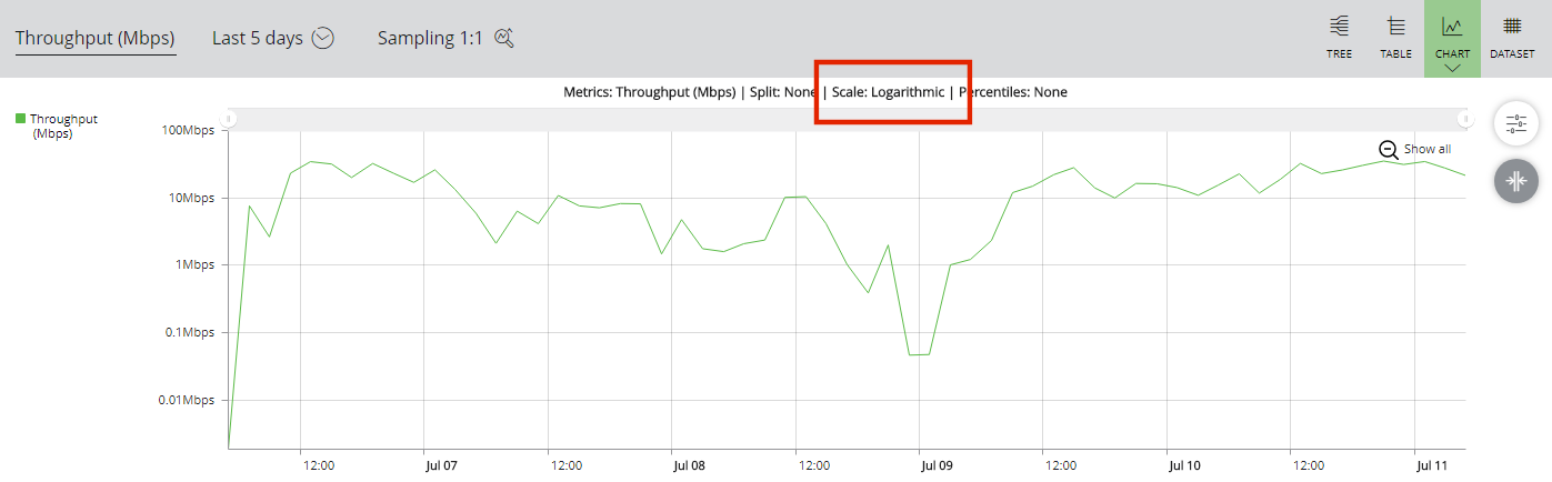
In this example:

•The vertical axis is marked from 0.01Mbps to 100Mbps, with each value ten times bigger than the last:

•0.01Mbps

•0.1Mbps

•1Mbps

•10Mbps

•100Mbps

•The smaller values are easier to read, because the logarithmic scale is more detailed at that level.

Assigning a Linear Scale or Logarithmic Axis Scale

To select the required axis scale:

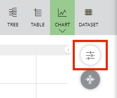
1.Click the Settings button.

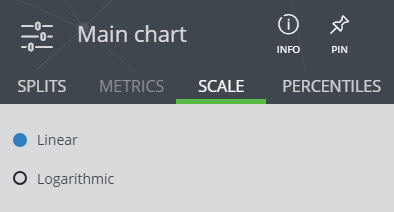
2.On the menu, select Scale.

The Main Chart settings panel appears with the Scale tab selected.

3.(Optional) click Pin to fix the panel to the side of the main display. This remains until unpinned.

4.Select the required axis scale, either:

•Linear

•Logarithmic

5.The Main Chart updates automatically.

Viewing Percentile Values

You can view percentile values within the main chart.

Percentiles are disabled when splits are in use, see Splitting the Primary Chart.

Some data metrics do not support percentiles. These metrics are disabled when percentiles are in use, see Viewing Percentile Values.

When you view percentiles, the main data line is replaced by three customizable percentile lines. By default, these lines are:

•The 99th percentile.

•The 95th percentile.

•The 50th percentile.

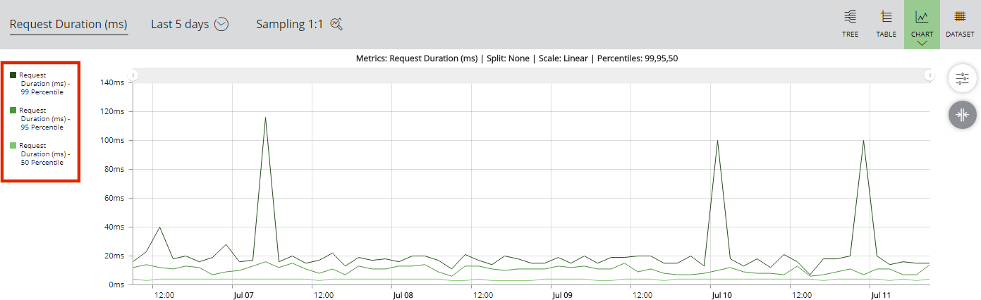
For example:

To replace the main data line by between one and three percentile lines on the main chart:

1.View the main chart. For example:

2.Click Settings for the main chart.

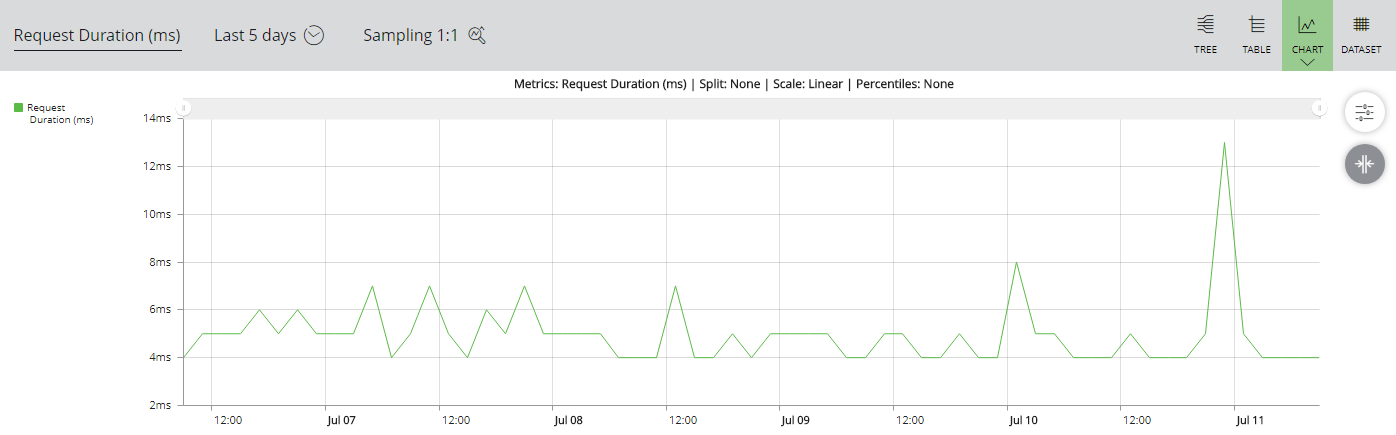
3.Select a chart metric that supports percentiles. That is, either:

•Request Duration (ms)

•Connection Duration (ms)

4.In the menu, select Percentile.

The Main Chart settings panel appears with the Percentiles tab selected.

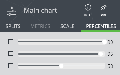
5.(Optional) click Pin to fix the panel to the side of the main display. This remains until unpinned.

6.Select the required number of percentiles.

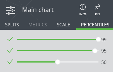
7.(Optional) Update the individual values of the enabled percentiles to a value between 1 and 100.

The main chart updates automatically.

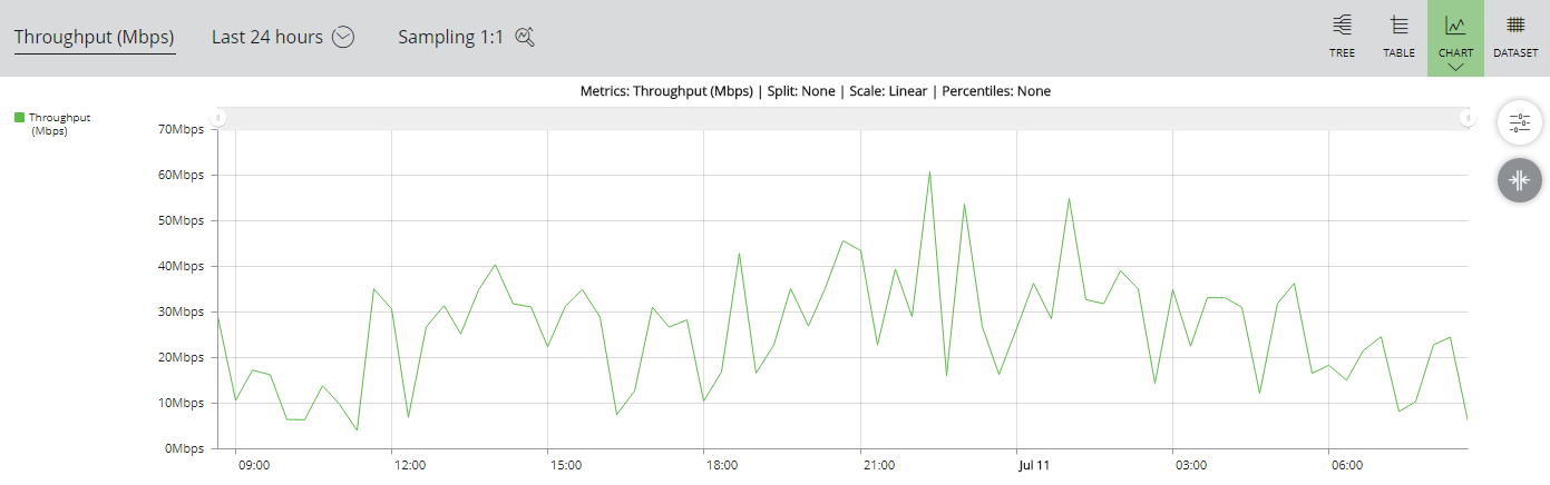
Working with the Primary Chart

The Primary Chart displays metrics over time. For example:

Where sampling is used, this is indicated by a smoothed curve.

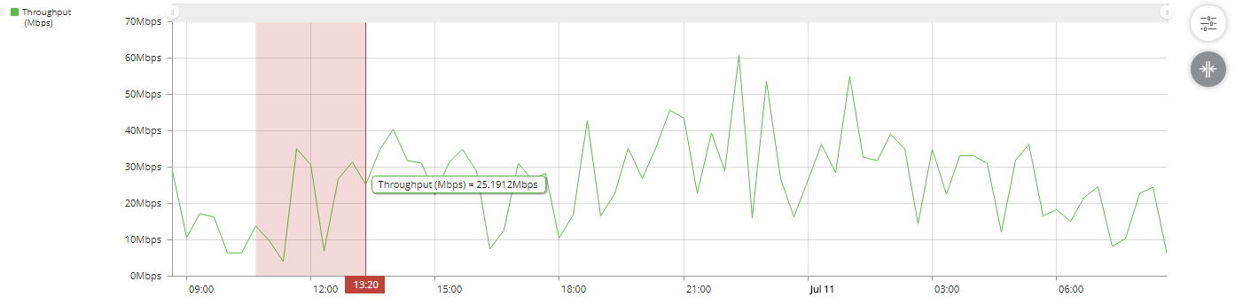
To examine data values for a point in time, hover the mouse pointer over a line.

Where sampling is used, this is indicated by an “approximately equal to" symbol, and an asterisk prefix for the value. For example:

Splitting the Primary Chart

Optionally, you can split the Primary Chart by component type. For example, If you split by vServer, each vServer has its own colour-coded line:

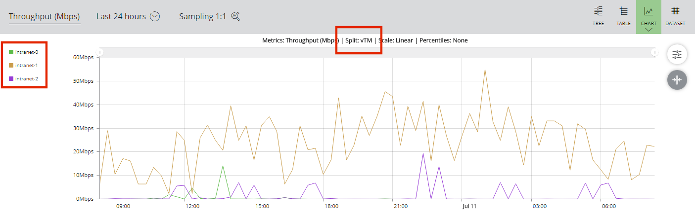
Where there are potentially more than ten lines, only the first ten are displayed individually. The data events from all remaining lines are aggregated as a single line named "Other".

When splits are used, bar charts are presented as stacked data.

When splits are used, percentiles are disabled. See Viewing Percentile Values.

To split the Primary Chart by a selected criteria:

1.Click the Settings button.

2.In the menu, select Splits.

The Main Chart panel appears.

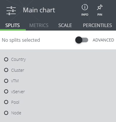
3.(Optional) click Pin to fix the panel to the side of the main display. This remains until unpinned.

4.Then, choose a split category. Either:

•If you want to split the Primary Chart using one of the basic component categories, select the Basic switch setting, and then select the required category. For example, vServer.

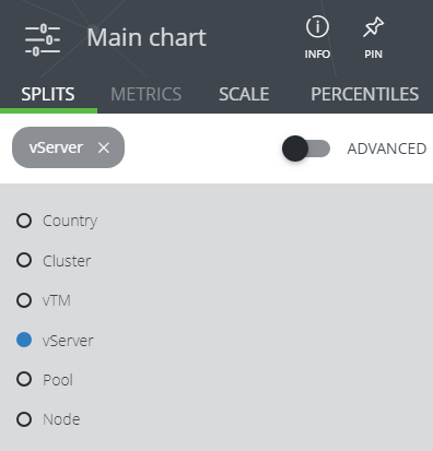
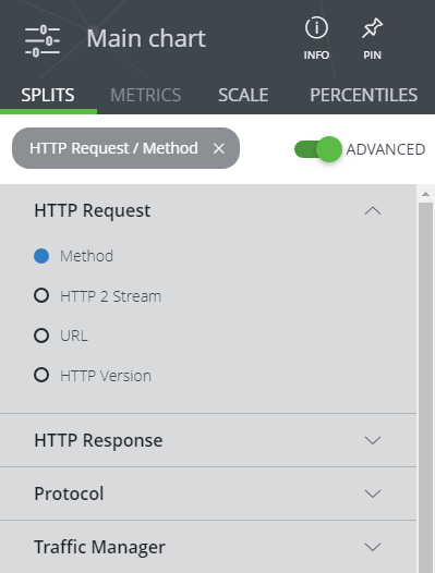
•If you want to split the Primary Chart using more specific criteria, select the Advanced switch setting.

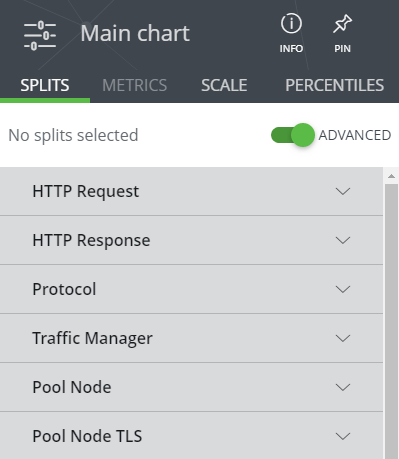
Then, locate and expand the required category, and select the required criteria. For example:

In both cases, once a selection is applied, the Primary Chart updates to reflect the selection.

Where there are potentially more than ten lines, only the first ten are displayed individually. The data events from all remaining lines are aggregated as a single line named "Other".

5.To examine data values for a point in time, hover the mouse pointer over the split lines. For example:

6.(Optional) To temporarily remove a split line from the display, click on its legend entry to the left of the graph. The line is then removed, and the graph is re-drawn. Click the legend again to re-include the line.

7.(Optional) To return to an un-split Primary Chart, delete the current selection on the Main Chart panel.

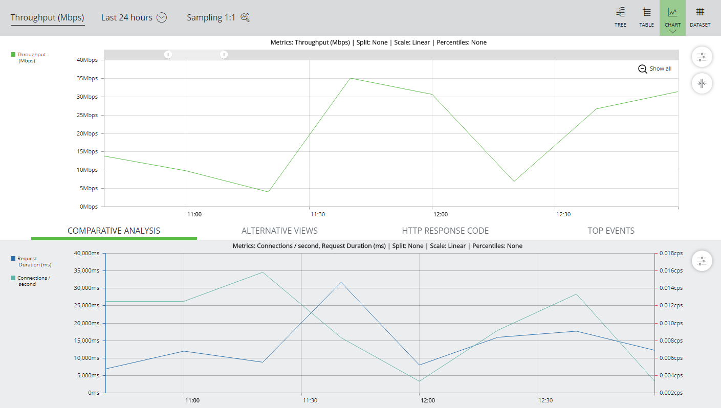
Focusing on a Time Range on the Primary Chart

You can focus the Primary Chart to a specific time range in the graph.

1.Display the Primary Chart (split if required). For example:

2.Drag across a time range in the graph. For example:

The graph updates to temporarily focus on the selected time range. The displayed section (a proportion within the original graph) is indicated by the sliders above the graph. For example:

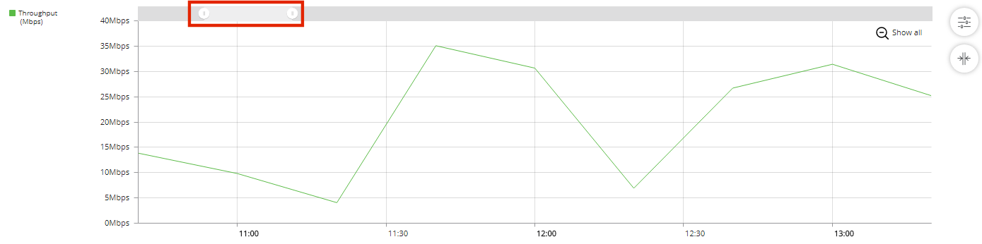
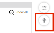
3.(Optional) Click the Focus button to permanently update the selected time range of the graph.

The position of each slider also updates.

4.(Optional) Click the Show All button to return the graph to its original time range.

The position of each slider also updates.

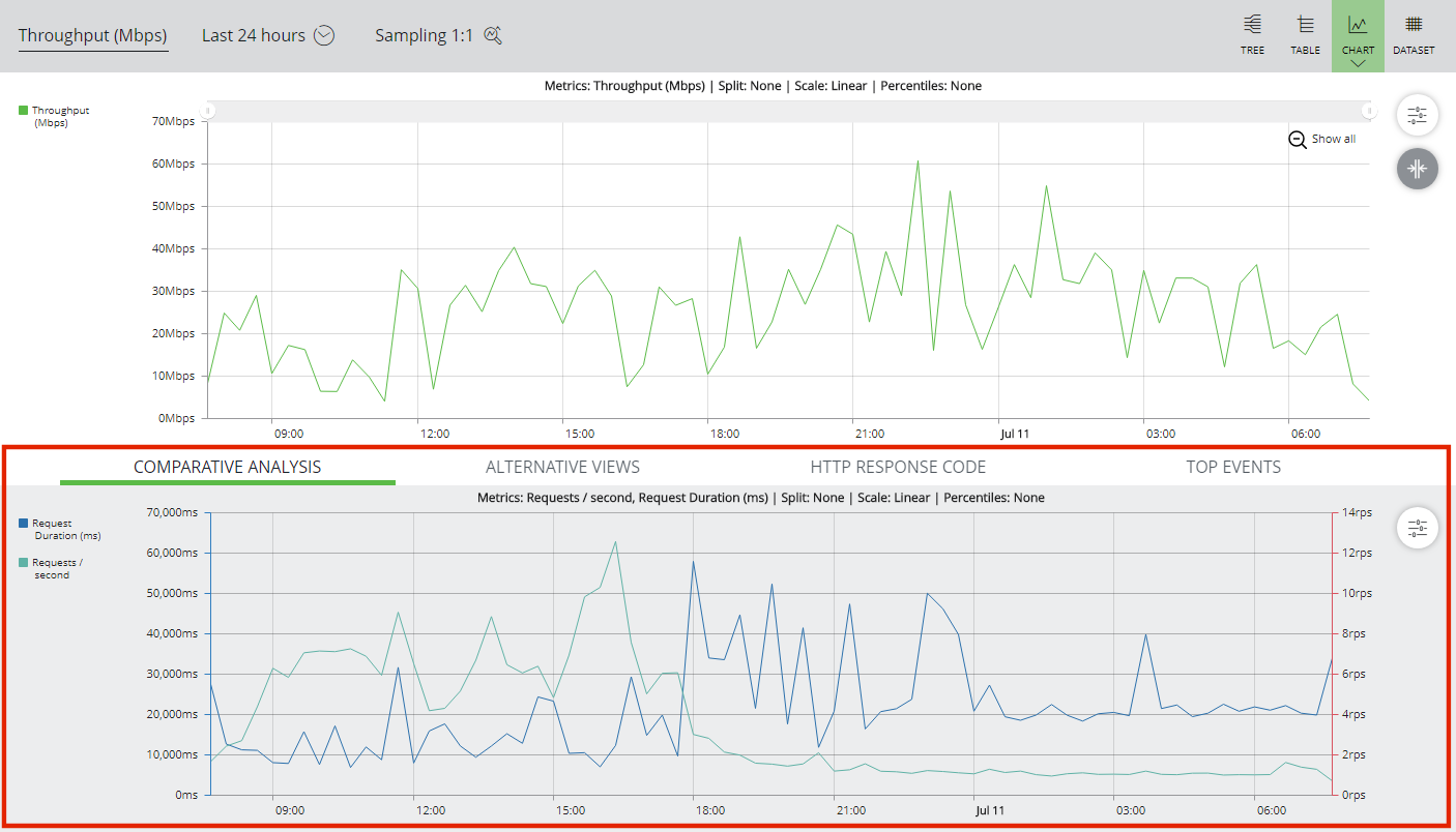
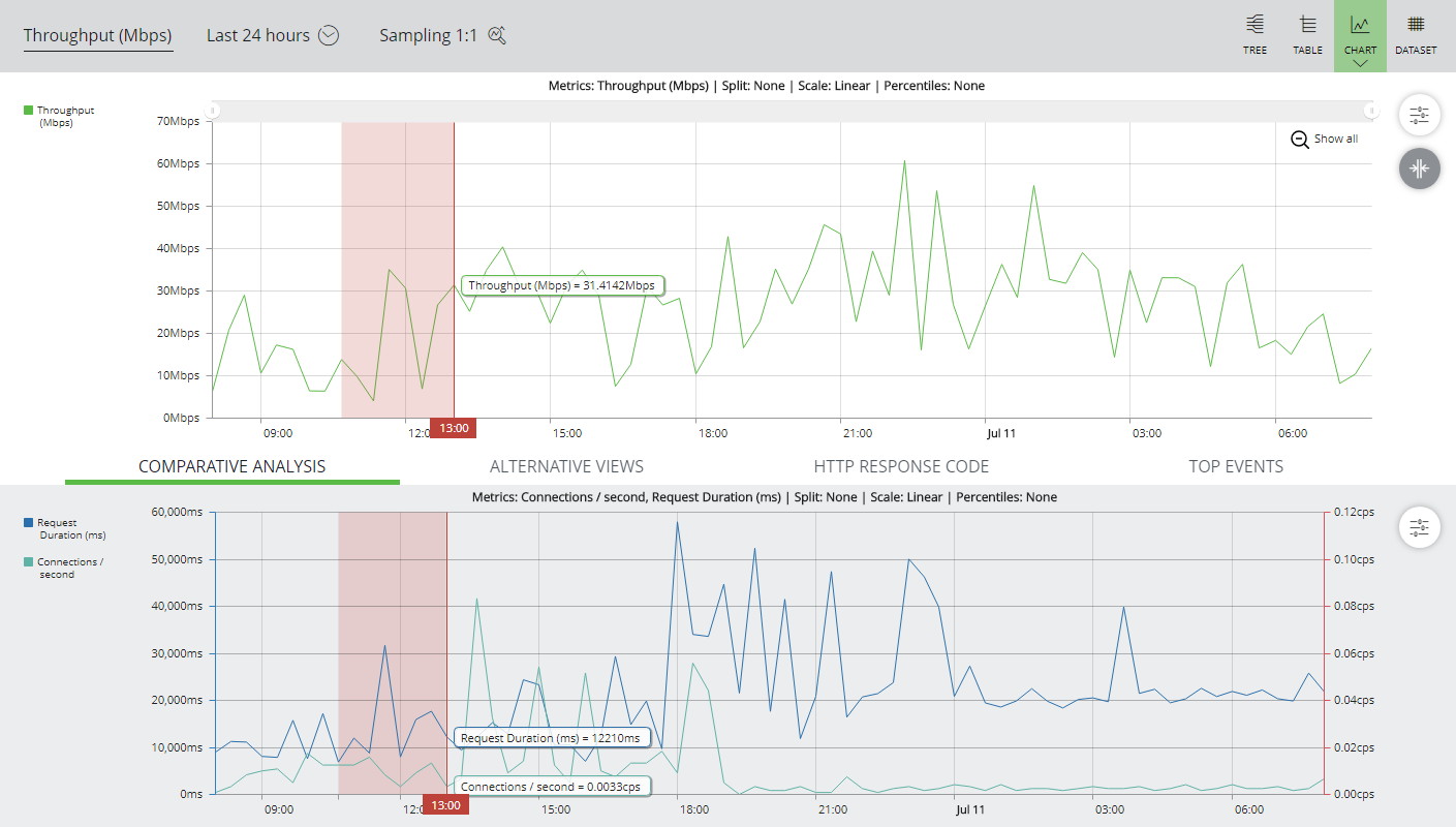
Performing Comparative Analysis

The Comparative Analysis tab enables you to view two different data metrics in a separate graph. This graph is based on the Primary Chart (see Starting the Chart). For example:

Control of the display settings for the Comparative Analysis graph is similar to that used on the main chart. However, splits and percentiles can only be applied when the comparative view contains a single data metric.

Creating a Comparative Analysis Graph

1.Display the Primary Chart, see Starting the Chart.

Do not split the Primary Chart. This is not supported by the Comparative Analysis graph.

2.Select the required time period for the Primary Chart, see Choosing a Time Period.

3.Select the required data metric for the Primary Chart, see Choosing a Data Metric.

4.(Optional) Set the Component Filter to include the required components, see Working with the Component Filter.

5.(Optional) Set the Extended Filter to include the required components, see Working with the Extended Filter.

6.Click the Comparative Analysis tab beneath the Primary Chart. The chart displays two charts, each based on a single default metric.

7.(Optional) To change the displayed metrics, click the Settings button in the Comparative Analysis tab.

8.In the menu, select Metrics.

The Comp. Analysis settings panel appears.

9.Click the Metrics tab selected. The two default metrics are indicated:

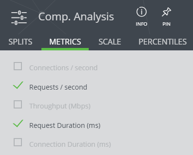
10.(Optional) click Pin to fix the panel to the side of the main display. This remains until unpinned.

11.(Optional) To switch one displayed metric for another, click the tick for a displayed metric.

Optionally, when you have a single data metric displayed in the Comparative Analysis graph, you can split the metric. You can also replace the data line with percentiles.

12.(Optional) Click the check box for the required second metric.

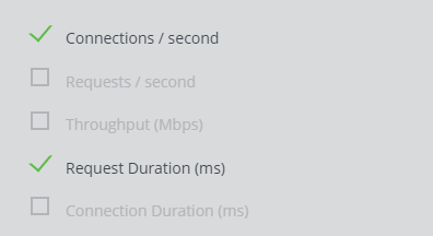
The Comparative Analysis graph updates.

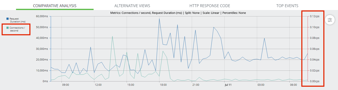
In this example, the Connections / Second data metric has been added. The data axis for this second metric is shown to the right of the Comparative Analysis Graph.

13.(Optional) Hover the mouse pointer over a data point in either graph to examine values in both graphs.

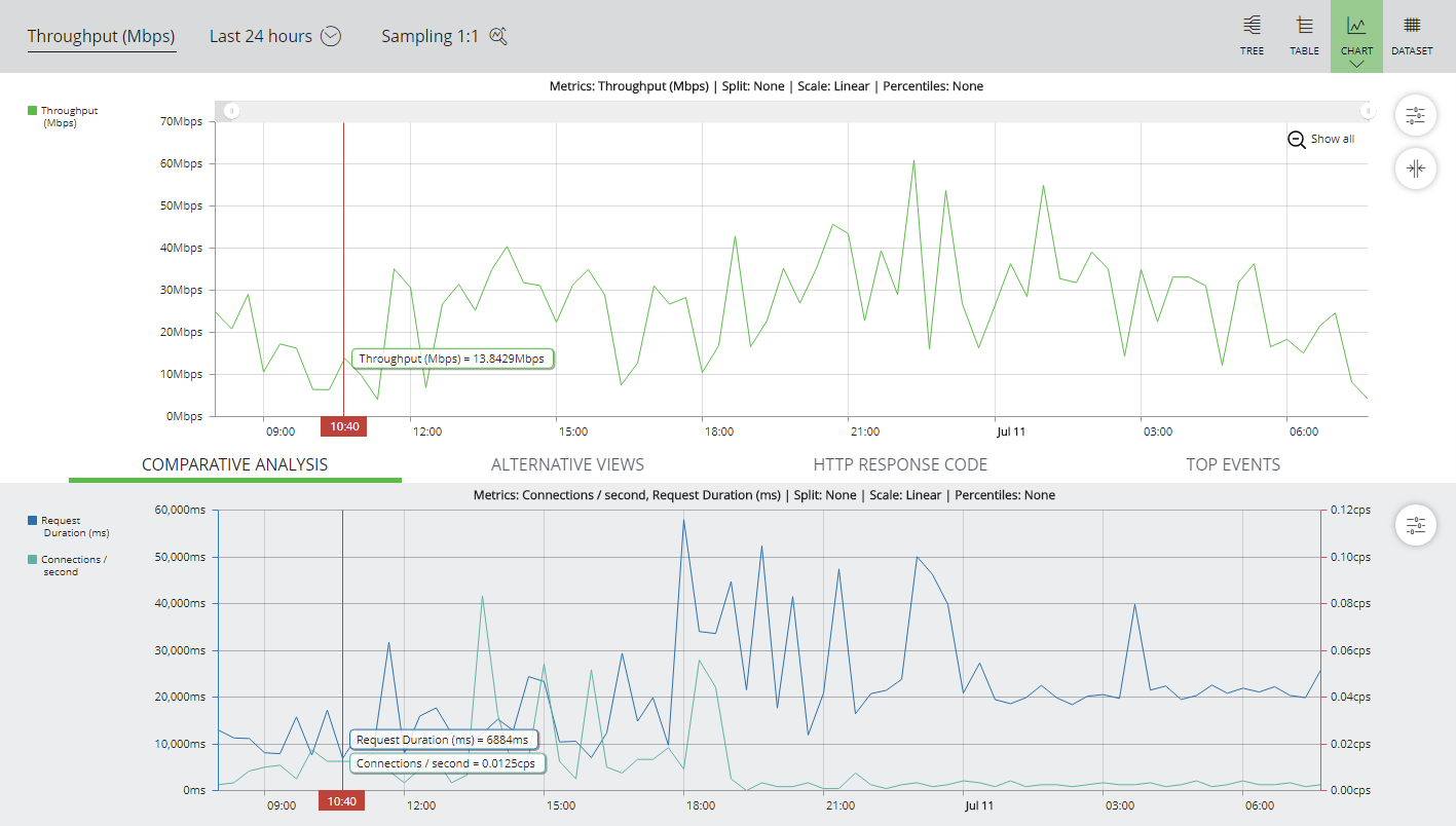
14.(Optional) Drag the mouse pointer over either graph to temporarily re-focus both graphs.

The graph updates to reflect the change.

The behaviour of this focused view is the same as that described in Focusing on a Time Range on the Primary Chart.

Viewing the Horseshoe Diagram

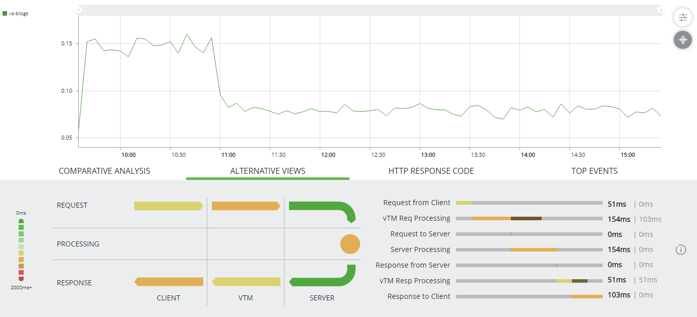
The Horseshoe Diagram displays average timings for various activities along the receive/transmit path for client requests, based on a single vServer. Colour coding is used. For example:

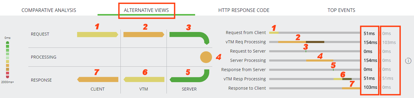
In this diagram, the numbers and boxes are superimposed. Descriptions are below.

The seven stages of the horseshoe diagram are:

1.Request from Client: The average time (in milliseconds) between the start and end of the client request reception on the vTM.

2.vTM Req Processing: The average time (in milliseconds) between the start of processing of the client request by the vTM, and the vTM being ready to communicate with the server. This time includes any TrafficScript processing that is required.

3.Request to Server: The average time (in milliseconds) between the start and end of the request being sent to the server for processing.

4.Server Processing: The average time (in milliseconds) for processing of the request by the server.

5.Response from Server: The average time (in milliseconds) between the start and end of the request being returned from the server.

6.vTM Resp Processing: The average time (in milliseconds) between the start of processing of the client response by the vTM. This time includes any TrafficScript processing that is required.

7.Response to Client: The average time (in milliseconds) between the start and end of the client response transmission from the vTM.

Next to the horseshoe diagram is a Gantt chart of timings. For each of the seven stages:

•The Timeline timing is for the part of the process that must complete before the vTM can begin processing the next stage. In generic Gantt chart terms, it indicates the critical path, and the colour associated with it is used for the matching section on the horseshoe diagram.

This timing is also displayed numerically in the first column to the right of the Gantt chart.

•The Overlap timing is for the remainder of a process after the next process starts. For example, HTTP client requests have both a request header and a request body, but vTM request processing can begin as soon as the request header is received. As such, the two processes overlap. In generic Gantt chart terms, it indicates a non-critical path, and (where present), it is coloured in a darker shade of the colour used for the Timeline timing. For example, see stage 2 and 3, above.

This timing is also displayed numerically in the second column to the right of the Gantt chart.

Creating a Horseshoe Diagram

1.Display the Primary Chart, see Starting the Chart.

2.Click the Alternative Views tab beneath the Primary Chart. For example:

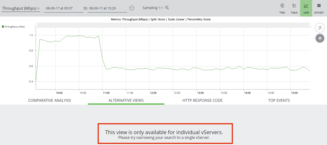
The Alternative Views tab requires a single selected vServer.

3.(Optional) Split the Primary Chart by vServer, see Splitting the Primary Chart. This enables you to view Charts for each vServer. For example:

4.Identify a single vServer using one of the following methods:

•Select the required vServer in the Component Filter, see Working with the Component Filter. OR

•Identify a single vServer using an Extended Filter clause, see Working with the Extended Filter. OR

•Hover the mouse pointer over the vServer lines in the Primary Chart. Then, select the required vServer by clicking on one of its data points.

After performing one of these methods, the Alternative Views tab updates to show the Horseshoe Diagram for the identified vServer. For example:

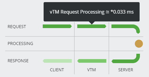
5.(Optional) Hover the mouse pointer over a section of the Horseshoe Diagram to see its value. For example:

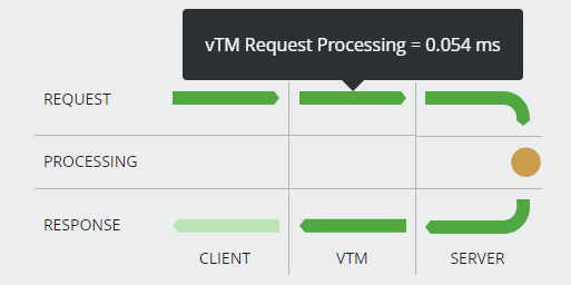
Where sampling is used, this is indicated by an asterisk prefix and an "approximately equal to" symbol. For example:

6.(Optional) To clear the selected vServer, expand the list of vServers in the Component Filter, and click Reset filter. See Working with the Component Filter.

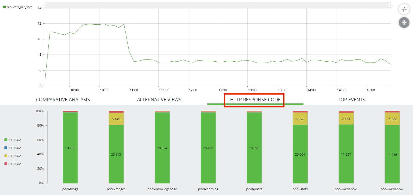
Viewing HTTP Response Codes

The HTTP Response Codes tab displays a bar chart that shows the HTTP Response codes received by the vTM pools present in the current Primary Chart. The response codes are percentage-based, and grouped into ranges of 100. For example:

Viewing Top Events

The Top Events tab displays stacked bar charts that shows HTTP Response codes for the vTM pools. The response codes are grouped into ranges of 100. For example:

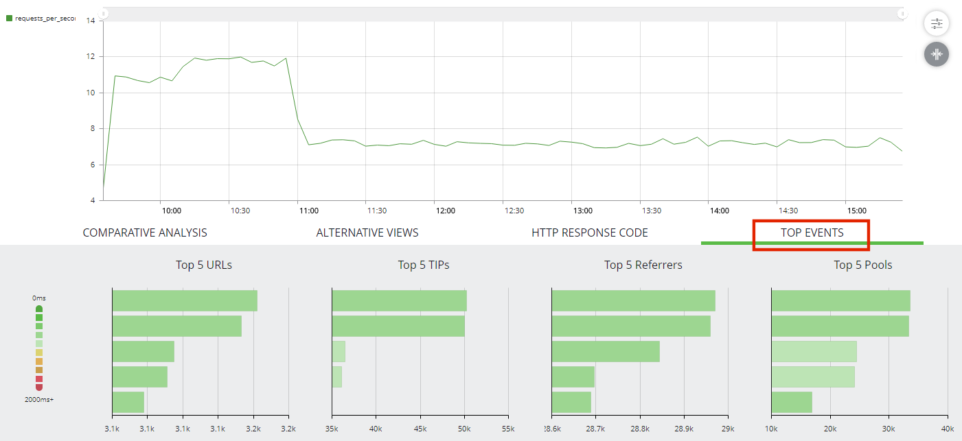
The displayed Top Event Graphs are:

•Top 5 URLs.

•Top 5 TIPs.

•Top 5 Referrers.

•Top 5 Pools.

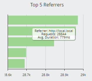
Hover the mouse pointer over any bar to view its details. For example:

When the Primary Chart is split, the bar charts are updated to results from the split category instead of the default pools.

When sampling is applied to the dataset, the entries and order of the entries in these graphs may vary between enquiries.

Using the Dataset View

The Dataset View displays the retrieved analytics data as individual rows of a table. For example:

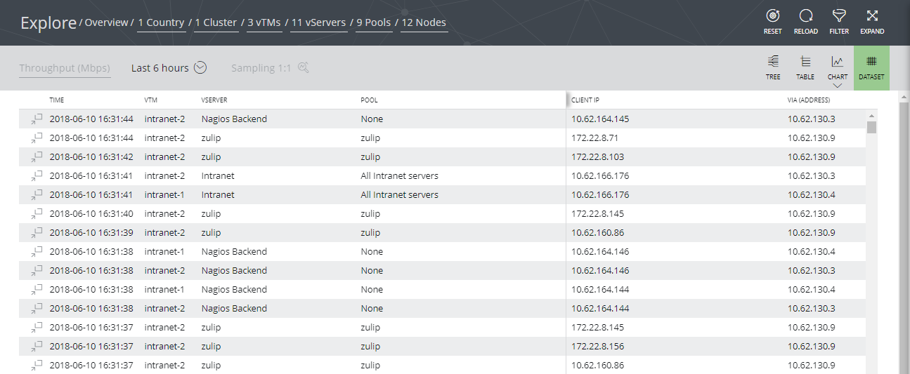
Sampling is never applied to the Dataset View.

The following properties are included for all data metrics:

•Time

•vTM

•vServer

•Pool

•Client IP

•Via

•Protocol

•Node

•Duration (ms)

•Bytes In

•Bytes Out

•Completion code

•HTTP method

•HTTP code

•HTTP URL

Starting the Dataset View

1.Start the vADC Analytics application, see Accessing the vADC Analytics Application.

2.Click Explore to access individual analytics graphs.

3.Finally, click the Dataset graph type.

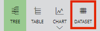
The Dataset View appears.

Viewing the Data for a Specific Row

You can view the underlying data that was used to create a specific row of the Dataset View.

1.Display the Dataset View, see Starting the Dataset View.

2.Locate and select the required row by clicking anywhere in the row.

The Display in Window button for the row activates (blue).

3.Click the Display in Window button.

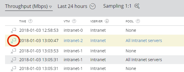
The Request Details window appears. This includes identifying information from the selected row.

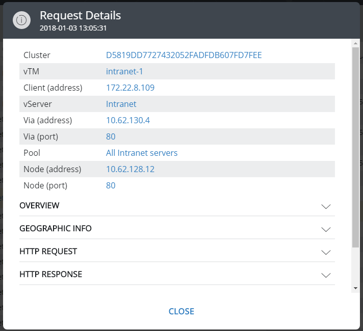
4.(Optional) Expand any of the sections to see the underlying data for the section:

•Overview

•Geographic Info

•HTTP Request

•HTTP Response

•Request Trace and Timeline

•Raw Data. This section includes entries that can be expanded to see deeper data.

Working with the Logs View

The Logs View displays retrieved log entries as individual rows of a table. For example:

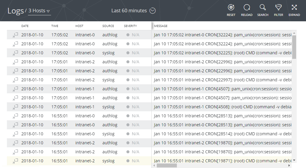
The following properties are included for each log entry:

•Date. The date of the log entry.

•Time. The time of the log entry.

•Host. The server that originated the log entry.

•Source. The log type for the log entry.

•Severity. The severity of the log entry.

•Message. The log message.

Starting the Logs View

1.Start the vADC Analytics application, see Accessing the vADC Analytics Application.

2.Click Logs to access the logs.

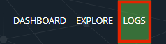
The Logs View appears.

Controlling the Logs View

You can control the display of logs in the following ways:

•You can select a specific originating host for log entries by selecting it from the Log Filter.

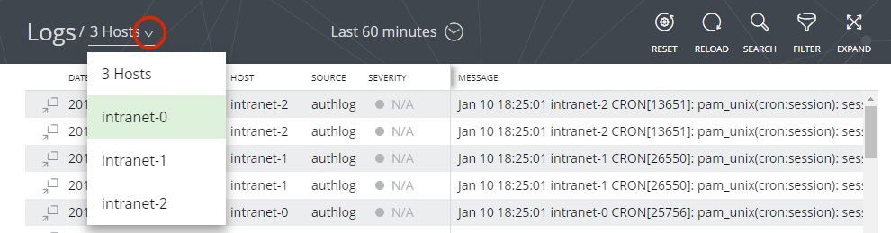
To reset the Log Filter, select the top listed item. In this example, after selecting the Intranet-0 host, you can then select 3 Hosts to revert to using all hosts.

•You can select a time period for displayed logs using the Time Selector. This operates in the same way as the Time Selector for graph types, see Choosing a Time Period.

•You can reset the Log Filter at any time by clicking the Reset button:

•You can refresh retrieved logs by clicking the Reload button. For example, to refresh the log data for the Last 60 minutes:

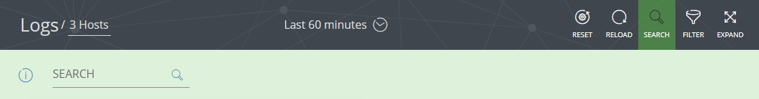
•You can search through log entries by clicking the Search button. See Searching in Displayed Logs for full details of this process.

•You can configure an extended set of filters in addition to the Component Filter by clicking the Filter button. This operates in the same way as the Extended Filter for graph types, see Working with the Extended Filter.

•You can maximize the use of space within the browser by clicking the Expand toggle.

Searching in Displayed Logs

You can search through the current displayed log entries using a text string.

1.To start a search, click Search.

The search text box appears.

2.Specify a search string. Searches are case-insensitive, and the following special characters are supported:

•* : A star matches zero or more characters, excluding whitespace unless the term is enclosed in double quotes. For example, use *.*.*.* to search for log entries that contain an IPv4 address.

•" : Use double quotes to enclose one or more spaces within a search term. For example, to search for the phrase session closed rather than log entries that contain the words session and closed, specify "session closed".

•- : A minus sign, used at the start of a search term (outside the double quotes if used), excludes all lines that contain the term. For example:

•To search for log entries that do not contain cron, specify -cron.

•To search for log entries that contain session but which do not contain closed, specify
session -closed".

•To search for log entries that do not contain the phrase session closed, specify -"session closed".

•\ : A backslash can be used to escape all special characters, including *, ", -, and itself.

For example, to search for -logind, specify \-logind

You can view this information by clicking the information button next to the search text box.

3.Press Enter or click the lens to search. For example:

The space-separated terms are then OR-ed together, except for negated terms which are AND-ed with the result of the non-negated terms. For example, to search for the word closed in a line that does not also contain the word session, specify session -closed.

After searching, the number of matching log entries is displayed and matching phrases are highlighted.

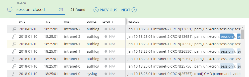
4.Click Next and Previous to navigate the located results.

5.(Optional) Click the Clear control to reset the search string. For example: